preface
After differential expression, most of us will see whether our differential gene screening can show the grouping results, and will choose the heat map, mainly the heat map skill clustering, which can also show the size of expression, which is very intuitive. Therefore, in this issue, we will talk about the drawing method of heat map.
Instance analysis
1. Data reading
We still use the data set of TCGA-COAD for data reading. We mentioned the reading of expression data and the acquisition of clinical information grouping in the previous period. We use the differential expression results calculated by edgeR software package and combine the original Count data, as follows:
DEG=read.table("DEG-resdata.xls",sep="\t",check.names=F,header = T)
PCAmat<-DEG[,8:ncol(DEG)]
rownames(PCAmat)=DEG[,1]
PCAmat[1:5,1:3]

##                 TCGA-3L-AA1B-01A-11R-A37K-07 TCGA-4N-A93T-01A-11R-A37K-07
## ENSG00000142959                           20                           15
## ENSG00000163815                          175                          108
## ENSG00000107611                           49                           13
## ENSG00000162461                           55                           89
## ENSG00000163959                          153                          259
##                 TCGA-4T-AA8H-01A-11R-A41B-07
## ENSG00000142959                           49
## ENSG00000163815                           59
## ENSG00000107611                            6
## ENSG00000162461                           48
## ENSG00000163959                          102
Read the grouping information, cancer tissue sample 478 and adjacent tissue sample 41, as follows:
group<-read.table("DEG-group.xls",sep="\t",check.names=F,header = T)
head(group)

##                         Sample Group
## 1 TCGA-D5-6530-01A-11R-1723-07    TP
## 2 TCGA-G4-6320-01A-11R-1723-07    TP
## 3 TCGA-AD-6888-01A-11R-1928-07    TP
## 4 TCGA-CK-6747-01A-11R-1839-07    TP
## 5 TCGA-AA-3975-01A-01R-1022-07    TP
## 6 TCGA-A6-6780-01A-11R-1839-07    TP
table(group$Group)

##
##  NT  TP
##  41 478
2. Convert count to FPKM
The data we downloaded earlier is Count, which is used for differential expression analysis. When drawing the heat map, we need to use RPKM or FPKM. Then we use the results of differential genes to extract the corresponding genes, get the Count matrix, download the gene length and calculate the FPKM. Remember the calculation formula of FPKM we talked about earlier,
FPKM (Fragments Per Kilobase of exon model per Million mapped fragments)
-
FPKM: transcripts per thousand bases, fragments per million mapped reads, mainly calculated for pair end sequencing expression.
-
The difference between FPKM and RPKM is that one is fragment and the other is read.
Then we first download the annotation information of exons. GDC reference files | NCI genetic data Commons (cancer. Gov) can find the following information and download it.
For the processing of exon annotation files, we want to get the gene length in the first column and the gene length in the second column.
Install and load the software package GenomicFeatures, which is very convenient for processing comment files, as follows:
if(!require(GenomicFeatures)){
  BiocManager::install("GenomicFeatures")
}

library(GenomicFeatures)
Read the downloaded annotation file and obtain the total length of exons, as follows:
txdb <- makeTxDbFromGFF("gencode.v22.annotation.gtf.gz",format = "gtf")
exons <- exonsBy(txdb,by="gene")


exons_length<-lapply(exons,function(x){sum(width(reduce(x)))})
class(exons_length)


## [1] "list"


length(exons_length)


## [1] 60483


exons_length<-as.data.frame(exons_length)
dim(exons_length)


## [1]     1 60483


exons_length1<-t(exons_length)
exons_length1<-as.data.frame(exons_length1)
dim(exons_length1)


## [1] 60483     1


head(exons_length1)


##                      V1
## ENSG00000000003.13 4535
## ENSG00000000005.5  1610
## ENSG00000000419.11 1207
## ENSG00000000457.12 6883
## ENSG00000000460.15 5967
## ENSG00000000938.11 3474
We found that there was no "." after the differential gene And numbers, so we need to remove the numbers behind the genes, as follows:
colnames(exons_length1)="Length"
Gene<-gsub("\\.(\\.?\\d*)","",rownames(exons_length1))
exons_length1$Gene=as.data.frame(Gene)[,1]
head(exons_length1)


##                    Length            Gene
## ENSG00000000003.13   4535 ENSG00000000003
## ENSG00000000005.5    1610 ENSG00000000005
## ENSG00000000419.11   1207 ENSG00000000419
## ENSG00000000457.12   6883 ENSG00000000457
## ENSG00000000460.15   5967 ENSG00000000460
## ENSG00000000938.11   3474 ENSG00000000938
The length of genes in the last column of the matrix is as follows:
PCAmat$Gene<-rownames(PCAmat)
####count matrix, length merging
count_length<-merge(PCAmat,exons_length1,by="Gene")
Calculate FPKM. According to the combined results, there are 519 samples, that is, from 2 columns to 520 columns. Calculate FPKM in combination with the formula, as follows:
kb<-count_length$Length/1000
countdata<-count_length[,2:520]
rpk <- countdata/kb
fpkm <-t(t(rpk)/colSums(countdata) * 10^6)
rownames(fpkm)=rownames(PCAmat)
fpkm[1:5,1:3]

##                 TCGA-3L-AA1B-01A-11R-A37K-07 TCGA-4N-A93T-01A-11R-A37K-07
## ENSG00000142959                    1.5336078                     1.826404
## ENSG00000163815                   51.1904250                   388.921103
## ENSG00000107611                  162.7697536                    52.262338
## ENSG00000162461                   69.9931252                    93.087394
## ENSG00000163959                    0.2628356                     0.000000
##                 TCGA-4T-AA8H-01A-11R-A41B-07
## ENSG00000142959                    0.7546987
## ENSG00000163815                  178.9371541
## ENSG00000107611                   13.3500151
## ENSG00000162461                   90.5084641
## ENSG00000163959                    0.0000000
The FPKM data is standardized as follows:
data=log2(fpkm+1)
dat=t(scale(t(data))) # 'scale 'can normalize the value of log(fpkm+1)
#Processing data
dat[dat>2]=2
dat[dat<(-2)]= -2
dim(dat)


## [1] 4128  519


dat[1:5,1:3]


##                 TCGA-3L-AA1B-01A-11R-A37K-07 TCGA-4N-A93T-01A-11R-A37K-07
## ENSG00000142959                  0.312929749                   0.51326990
## ENSG00000163815                 -0.451067532                   1.30683599
## ENSG00000107611                  0.811371990                   0.01667015
## ENSG00000162461                 -0.076316888                   0.23114035
## ENSG00000163959                 -0.004643292                  -0.62802639
##                 TCGA-4T-AA8H-01A-11R-A41B-07
## ENSG00000142959                   -0.3600191
## ENSG00000163815                    0.6308436
## ENSG00000107611                   -0.9112186
## ENSG00000162461                    0.2008002
## ENSG00000163959                   -0.6280264
3. Draw heat map
The software package pheatmap is used for heat map drawing. This software package is very convenient to use and has many parameters, which can meet various needs. More importantly, it can extract clustering data and process clustering results twice by itself, which is convenient for annotation.
Install and load the software package as follows:
if(!require(pheatmap)){
  install.packages("pheatmap")
}

library(pheatmap)
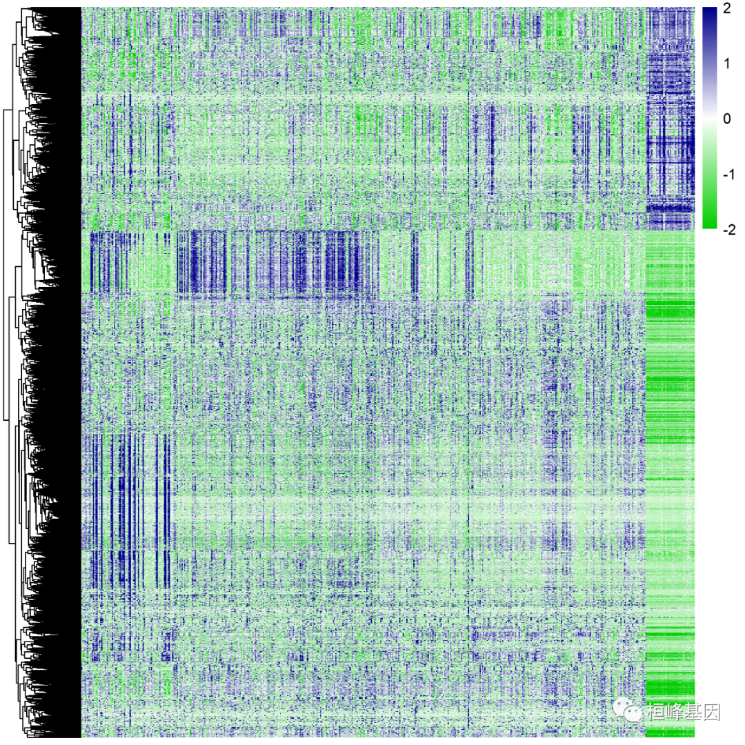
The simplest way to draw a heat map is as follows:
###########pheatmap
#Adjust parameters and change color
pheatmap(dat,
         cluster_rows = TRUE,
         show_rownames=FALSE,
         show_colnames = FALSE,
          scale="none",
          cluster_cols = F,
          fontsize_row = 10,
          fontsize_col = 10,
          #color = colorRampPalette(c("navy", "white", "firebrick3"))(100),
          color = colorRampPalette(c("green3", "white", "blue4"))(100),#Change color
          angle_col = 45, #Change the inclination of the horizontal axis coordinate name
          filename = 'cor.fpkm1.png',
)
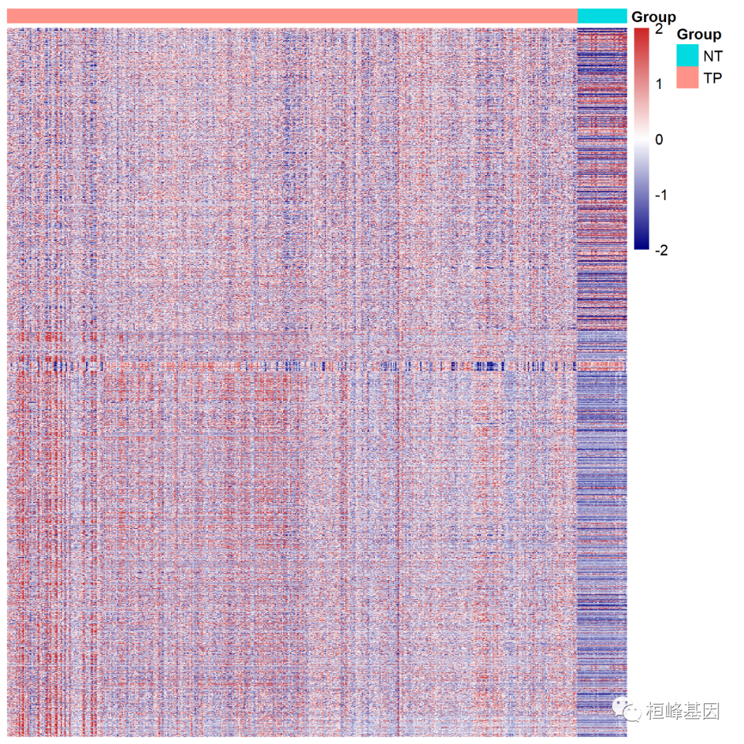
To add annotation information, you need to make a group information,
The first is the grouping annotation of samples, which is sorted according to cancer group and normal group, that is, column annotation data processing, as follows:
#######Annotated information
rownames(group)=group$Sample
head(group)

##                                                    Sample Group
## TCGA-D5-6530-01A-11R-1723-07 TCGA-D5-6530-01A-11R-1723-07    TP
## TCGA-G4-6320-01A-11R-1723-07 TCGA-G4-6320-01A-11R-1723-07    TP
## TCGA-AD-6888-01A-11R-1928-07 TCGA-AD-6888-01A-11R-1928-07    TP
## TCGA-CK-6747-01A-11R-1839-07 TCGA-CK-6747-01A-11R-1839-07    TP
## TCGA-AA-3975-01A-01R-1022-07 TCGA-AA-3975-01A-01R-1022-07    TP
## TCGA-A6-6780-01A-11R-1839-07 TCGA-A6-6780-01A-11R-1839-07    TP


group1=group[colnames(dat),-1,drop=FALSE]
head(group1)


##                              Group
## TCGA-3L-AA1B-01A-11R-A37K-07    TP
## TCGA-4N-A93T-01A-11R-A37K-07    TP
## TCGA-4T-AA8H-01A-11R-A41B-07    TP
## TCGA-5M-AAT4-01A-11R-A41B-07    TP
## TCGA-5M-AAT5-01A-21R-A41B-07    TP
## TCGA-5M-AAT6-01A-11R-A41B-07    TP
Add column notes, and then draw the heat map, as follows:
pheatmap(dat,
         cluster_rows = FALSE,
         show_rownames=FALSE,
         show_colnames = FALSE,
         scale="none",
         cluster_cols = FALSE,
         fontsize_row = 10,
         fontsize_col = 10,
         annotation_col = group1,
         color = colorRampPalette(c("navy", "white", "firebrick3"))(100),
         #color = colorRampPalette(c("green3", "white", "blue4"))(100),#Change color
         angle_col = 45, #Change the inclination of the horizontal axis coordinate name
         filename = 'cor.fpkm2.png',
)
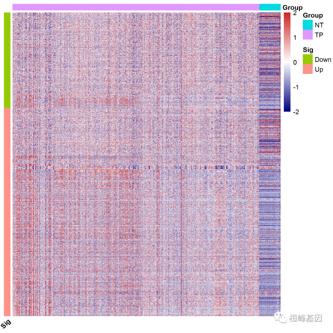
Adjust the sequence of genes according to the grouping of Up and Down in the difference results, and process the lines. This is actually a grouping of genes, which are divided into Up and Down, as follows:
ann_row=as.data.frame(DEG[,c(1,7)])
colnames(ann_row)=c("Sample","Sig")
rownames(ann_row)=DEG$Row.names
ann_row=ann_row[order(ann_row$Sig),]
rownames(ann_row)=ann_row$Sample
ann_row=as.data.frame(ann_row)
ann_row1=as.data.frame(ann_row[,2])
rownames(ann_row1)=ann_row$Sample
colnames(ann_row1)="Sig"
head(ann_row1)


##                  Sig
## ENSG00000142959 Down
## ENSG00000163815 Down
## ENSG00000107611 Down
## ENSG00000162461 Down
## ENSG00000163959 Down
## ENSG00000144410 Down
Add row and column notes, and then draw the heat map, as follows:
#######Adjust the sequence of genes according to the grouping of up and down in the difference results
pheatmap(dat[rownames(ann_row1),],
         cluster_rows = FALSE,
         show_rownames=FALSE,
         show_colnames = FALSE,
         scale="none",
         cluster_cols = FALSE,
         fontsize_row = 10,
         fontsize_col = 10,
         annotation_col = group1,
         annotation_row = ann_row1,
         color = colorRampPalette(c("navy", "white", "firebrick3"))(100),
         #color = colorRampPalette(c("green3", "white", "blue4"))(100),#Change color
         angle_col = 45, #Change the inclination of the horizontal axis coordinate name
         filename = 'cor.fpkm3.png',
)
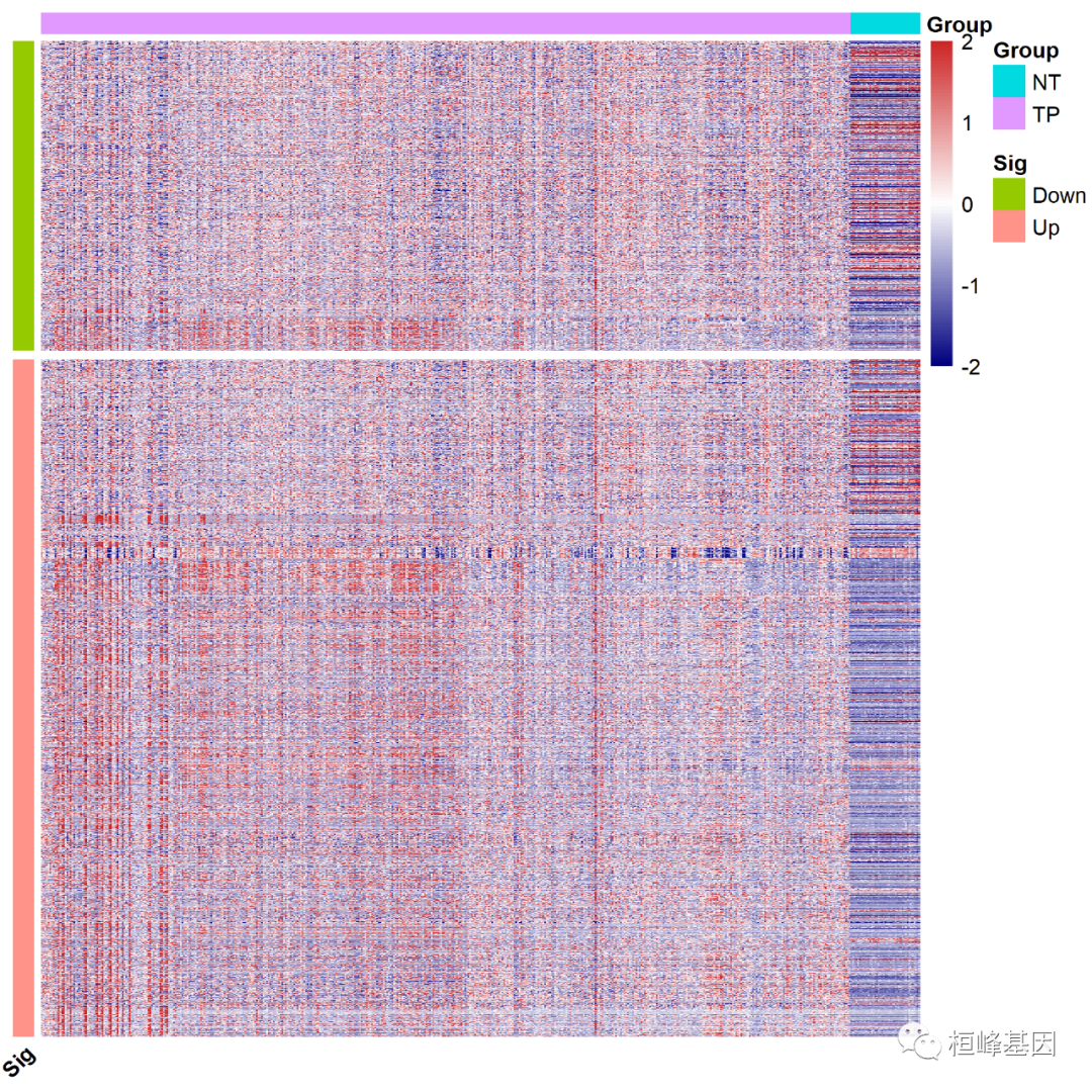
Split multiple modules. Let's first look at the number of genes up and down regulated. The number of genes down regulated is 1296, as follows
table(ann_row1$Sig)


##
## Down   Up
## 1296 2832
Set gaps according to the number of down regulated genes_ Row = 1296, as follows:
#########Split multiple modules
pheatmap(dat[rownames(ann_row1),],
         cluster_rows = FALSE,
         show_rownames=FALSE,
         show_colnames = FALSE,
         scale="none",
         cluster_cols = FALSE,
         fontsize_row = 10,
         fontsize_col = 10,
         annotation_col = group1,
         annotation_row = ann_row1,
         color = colorRampPalette(c("navy", "white", "firebrick3"))(100),
         #color = colorRampPalette(c("green3", "white", "blue4"))(100),#Change color
         angle_col = 45, #Change the inclination of the horizontal axis coordinate name
         filename = 'cor.fpkm4.png',
         gaps_row=1296#Split position
)
It is very simple, but we need to carefully prepare data, pay attention to the official account, scan the code into groups, and keep the exciting content updated.

Huanfeng gene
Bioinformatics analysis, SCI article writing and bioinformatics basic knowledge learning: R language learning, perl basic programming, linux system commands, Python meet you better
45 original content
official account