The most complete GO annotation result drawing in the whole network, directly click the SCI drawing annotation, pay attention to me, your best choice!
preface
1. GO principle
Genome sequencing has shown that most genes that specify core biological functions are common to all eukaryotes. This knowledge can often be transferred from one organism to other organisms. The goal of gene ontology alliance is to produce a dynamic and controllable vocabulary that can be applied to all eukaryotes, even if the knowledge of the role of genes and proteins in cells is accumulating and changing. To this end, three independent ontologies can be accessed on the Web all over the world.
When we get a project of non model organisms or no reference genome, we often need to annotate the function of genes before we can analyze the data of bioinformatics. Although, ah, the functions of genes with similar sequences are often conservative in different species, in the past, there were often different descriptions of the functions of the same genes in different laboratories because of the fuzziness of our natural language. Obviously, we need a unified term to describe the functions of these cross species homologous genes and their gene products, otherwise this ambiguity will greatly limit the academic communication between different researchers.
With the accumulation of bioinformatics data, there are different classification databases used to describe gene function. The goal of these classification systems is to elaborate the biological functions of these cross species homologous genes. However, because the results of gene function annotation between classification systems may be different in natural language description, and they are all their own dialects, most classification results can hardly be translated directly between classification systems. The Gene Ontology (GO) project is the result of efforts to make the functional description of gene products obtained by genes in various databases consistent.
In the GO classification system, there are three basic classifications (officially called the namespace of entries):
-
cellular component: each part of the cell and the extracellular environment.
-
molecular function: it can be described as activity at the molecular level, such as catalytic or binding activity.
-
Biological process: biological process refers to a series of events generated by the orderly combination of one or more molecular functions.
Similar to GO classification, another attempt to clarify the essence of biological function is the relatively early birth of the very classic NCBI lineal homologous protein cluster, namely cog classification (COG is also divided into four versions: prokaryotic bacterial branch is cog, eukaryotic branch is KOG, archaeal branch is arCOG and phage branch is POG). The cog classification system has the following four basic classifications:
-
INFORMATION STORAGE AND PROCESSING
-
CELLULAR PROCESSES AND SIGNALING
-
Metabolically related (METABOLISM)
-
Difficult to classify
Another very important KEGG lineal homology for gene function classification in the system field is further subdivided into seven basic functional classifications compared with COG classification:
-
Metabolism related
-
Genetic Information Processing
-
Environmental Information Processing
-
Intracellular processes
-
Organic systems
-
Human Diseases
-
Not Included in Pathway or Brite
Gene Ontology is only from the full name of go Gene Ontology. GO annotation system is a classification system established to elaborate the essential attributes of biological macromolecules, where essential attributes refer to biological functions. Go classification uses four elements to describe the essential information of gene units:
-
concepts: an essential concept is our description of the functional annotation results of a gene and its products. In GO annotation, a concept is a Term entry specific to a GO id number.
-
Relationship: in the Go annotation system, there can be an is between two entries_ a,part_of,has_part and regulations. If we regard the entry as a node and the relationship between entries as an edge connection between two nodes, we can build a directed acyclic graph based on many nodes or a relational network.
-
Instances: instances are biological macromolecules that play specific biological functions in life activities, such as proteins with GO annotation information. In UniProt protein database, all protein sequences with UniProt number are the target instance object of GO annotation.
-
axioms: Axiomatic inference rules are the most important rules in the GO annotation system to explain the essential concept. axioms refer to the rules for inferring the relationship between entries, such as a is_ A, B, and B is_a C, then we can infer A is_a C, the inference rule information used in the process of inferring a to C, is an axiom. Because we infer a is from the relationship_ A C, so C is the essence of A. similarly, C is also the essence of B.
2. Example analysis
1. Data reading
We still use the data set of TCGA-COAD for data reading. We mentioned the reading of expression data and the acquisition of clinical information grouping in the previous period. We use the differential expression results calculated by edgeR software package to extract the ENSEMBL number of up-regulated gene 2832,
###########Gene list
DEG=read.table("DEG-resdata.xls",sep="\t",check.names=F,header = T)
geneList<-DEG[DEG$sig=="Up",]$Row.names
table(DEG$sig)

##
## Down   Up
## 1296 2832
Read the sample grouping information, 41 normal tissues and 478 cancer tissues, as follows:
######Sample grouping information
group<-read.table("DEG-group.xls",sep="\t",check.names=F,header = T)
table(group$Group)


##
##  NT  TP
##  41 478
2. GO annotation results
First, we also need to install the software package and load it. The main program is the clusterProfiler software package, as follows:
if(!require(clusterProfiler)){
  BiocManager::install("clusterProfiler")
}
if(!require(org.Hs.eg.db)){
  BiocManager::install("org.Hs.eg.db")
}
if(!require(DOSE)){
  BiocManager::install("DOSE")
}
if(!require(topGO)){
  BiocManager::install("topGO")
}
if(!require(pathview)){
  BiocManager::install("pathview")
}
library(org.Hs.eg.db)
library(clusterProfiler)
library(DOSE)
library(topGO)
library(pathview)
According to the data comparison, we found some genes in 1726 GO data. At the same time, we obtained three naming methods of a gene, namely "ENTREZID", "ENSEMBL", "SYMBOL", as follows:
eg <- bitr(geneList,
           fromType="ENSEMBL",
           toType=c("ENTREZID","ENSEMBL",'SYMBOL'),
           OrgDb="org.Hs.eg.db")


## 'select()' returned 1:many mapping between keys and columns


## Warning in bitr(geneList, fromType = "ENSEMBL", toType = c("ENTREZID",
## "ENSEMBL", : 39.51% of input gene IDs are fail to map...

dim(eg)

## [1] 1726    3


head(eg)

##           ENSEMBL ENTREZID  SYMBOL
## 1 ENSG00000062038     1001    CDH3
## 2 ENSG00000175832     2118    ETV4
## 3 ENSG00000167767   144501   KRT80
## 4 ENSG00000164283    11082    ESM1
## 5 ENSG00000120254    25902 MTHFD1L
## 6 ENSG00000129474    84962   AJUBA
GO annotation is carried out for the obtained genes. The ont parameters have four selection modes, ALL, MF, CC and BP, among which (MF, CC and BP) are the three basic classifications we mentioned above. In the go classification system, there are three basic classifications, and ALL annotates these three classifications at the same time. We select "ALL" here, and the thresholds are pvvaluecutoff = 0.01 and qvalueCutoff = 0.05 respectively, During annotation, we can select three different gene names in the parameter keyType, as follows:
# Run GO enrichment analysis
go <- enrichGO(eg$SYMBOL,
               OrgDb = org.Hs.eg.db,
               ont='ALL',
               keyType = "SYMBOL",
               pAdjustMethod = 'BH',
               pvalueCutoff = 0.01,
               qvalueCutoff = 0.05,
               #keyType = 'ENTREZID'
)
dim(go)


## [1] 232  10
Look at the final results and keep the results. We can see that BP, CC and MF are 193, 10 and 29 respectively, as follows:
head(go@result)

##            ONTOLOGY         ID
## GO:0007389       BP GO:0007389
## GO:0019730       BP GO:0019730
## GO:0061844       BP GO:0061844
## GO:0003002       BP GO:0003002
## GO:0048568       BP GO:0048568
## GO:0045165       BP GO:0045165
##                                                                        Description
## GO:0007389                                           pattern specification process
## GO:0019730                                          antimicrobial humoral response
## GO:0061844 antimicrobial humoral immune response mediated by antimicrobial peptide
## GO:0003002                                                         regionalization
## GO:0048568                                             embryonic organ development
## GO:0045165                                                    cell fate commitment
##            GeneRatio   BgRatio       pvalue     p.adjust       qvalue
## GO:0007389    64/927 436/18722 4.639425e-15 2.023253e-11 1.787888e-11
## GO:0019730    31/927 122/18722 2.490775e-14 5.431135e-11 4.799330e-11
## GO:0061844    24/927  79/18722 2.963461e-13 4.307885e-10 3.806748e-10
## GO:0003002    51/927 331/18722 4.507505e-13 4.914307e-10 4.342625e-10
## GO:0048568    57/927 427/18722 8.233615e-12 6.338388e-09 5.601042e-09
## GO:0045165    42/927 258/18722 8.720552e-12 6.338388e-09 5.601042e-09
##                                                                                                                                                                                                                                                                                                                                                                        geneID
## GO:0007389 WNT2/SIM2/OTX1/MDFI/XRCC2/GRHL3/WNT3/MSX1/FEZF1/CFAP45/SHH/WNT7B/LEF1/NKD1/AXIN2/GBX2/TDGF1/SIX1/STC1/WT1/DNAH5/HOXB8/RIPPLY3/BMP7/CITED1/FOLR1/DMRTA2/TDGF1P3/DMRT3/WNT8B/IRX3/SP8/RIPPLY1/HES7/WNT11/SOX1/ROBO2/DLL3/FGF8/DKK1/FOXD1/SIX2/EYA1/GSC/LRP2/TBX20/NODAL/NKX2-1/SIX3/GATA4/PAX2/WNT3A/FEZF2/LHX1/IRX2/NKX2-5/EN1/LHX3/TBX5/WNT7A/NTF4/FOXG1/TBR1/IRX4
## GO:0019730                                                                                                                                                                     KLK7/CXCL3/CXCL1/SLC11A1/CXCL2/PGC/CXCL8/CXCL5/PPBP/WFDC10A/F2/WFDC10B/CXCL6/KRT6A/CXCL11/PGLYRP3/H2BC10/H2BC6/PRSS2/H2BC7/S100A7/IL36RN/FGB/PGLYRP4/IL17A/H2BC11/SEMG1/KLK5/SEMG2/REG3A/IL17F
## GO:0061844                                                                                                                                                                                                                    KLK7/CXCL3/CXCL1/CXCL2/PGC/CXCL8/CXCL5/PPBP/F2/CXCL6/KRT6A/CXCL11/PGLYRP3/H2BC10/H2BC6/H2BC7/S100A7/PGLYRP4/IL17A/H2BC11/SEMG1/KLK5/REG3A/IL17F
## GO:0003002                                                                              WNT2/OTX1/MDFI/XRCC2/WNT3/MSX1/FEZF1/SHH/WNT7B/LEF1/NKD1/AXIN2/GBX2/TDGF1/SIX1/WT1/HOXB8/DMRTA2/TDGF1P3/DMRT3/WNT8B/IRX3/SP8/RIPPLY1/HES7/WNT11/SOX1/ROBO2/DLL3/FGF8/DKK1/FOXD1/SIX2/GSC/LRP2/TBX20/NODAL/NKX2-1/SIX3/GATA4/PAX2/WNT3A/FEZF2/LHX1/IRX2/EN1/LHX3/WNT7A/NTF4/FOXG1/TBR1
## GO:0048568                                          MTHFD1L/WNT2/OTX1/MDFI/TEAD4/COL11A1/CTHRC1/STRA6/GRHL3/MSX1/ASCL2/IRX5/APELA/SHH/WNT7B/MFAP2/LEF1/GBX2/TFAP2A/SIX1/TBX15/PTK7/HOXB8/BMP7/EN2/CXCL8/SIX4/CSF2/CITED1/FOLR1/GJB5/TH/IGF2/MYCN/WNT11/DLX6/FGF8/ATP6V1B1/SIX2/EYA1/GSC/TBX4/TBX20/NODAL/SHOX2/SIX3/DLX5/GATA4/GJB6/GCM1/PAX2/WNT3A/LHX1/HPN/NKX2-5/EN1/FOXG1
## GO:0045165                                                                                                                        WNT2/EPOP/WNT3/SHH/WNT7B/IL23A/SIX1/WT1/TBX15/ONECUT2/DMRTA2/DMRT3/WNT8B/POU3F2/WNT11/SOX1/FGF8/DKK1/POU4F1/SIX2/EYA1/GSC/TBX4/TBX20/NODAL/PTF1A/NKX2-1/GATA4/GCM1/PAX2/WNT3A/GSX1/FEZF2/POU6F2/TLX3/LHX3/TBX5/WNT7A/NTF4/FOXG1/TBR1/NKX6-3
##            Count
## GO:0007389    64
## GO:0019730    31
## GO:0061844    24
## GO:0003002    51
## GO:0048568    57
## GO:0045165    42


table(go@result$ONTOLOGY)
##
##  BP  CC  MF
## 193  10  29
3. Result display
For the GO annotation results, we give a variety of display methods here. According to our own needs and the design of the article, we can choose the one suitable for ourselves.
library(stringr)
library(cowplot)
library(ggplot2)
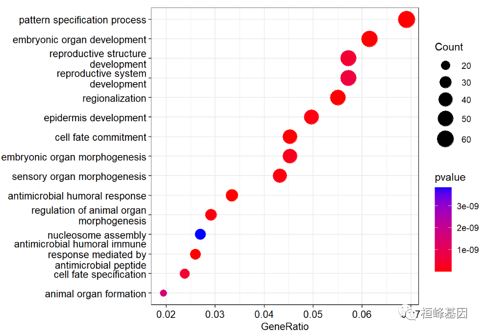
Draw a bubble chart. The interpretation of the bubble chart needs to explain that the enrichment degree of GO is measured by Gene ratio, Pvalue and the number of genes enriched on this GO term.
-
The abscissa is Gene ratio. The greater the value, the greater the enrichment degree. Count the number of differentially expressed genes under the GO term
-
The ordinate is the GO term with high enrichment degree (generally, 20 items with the most significant enrichment are selected for display, and less than 20 items are listed).
-
The value range of Pvalue [0, 1] is expressed in color. The redder it is, the smaller Pvalue is, indicating that the enrichment is more obvious.
-
The size of the dot indicates the number of differential genes under the term. The larger the dot, the more genes.
dotplot(go,
        showCategory=15,
        font.size=10,
        color ="pvalue")
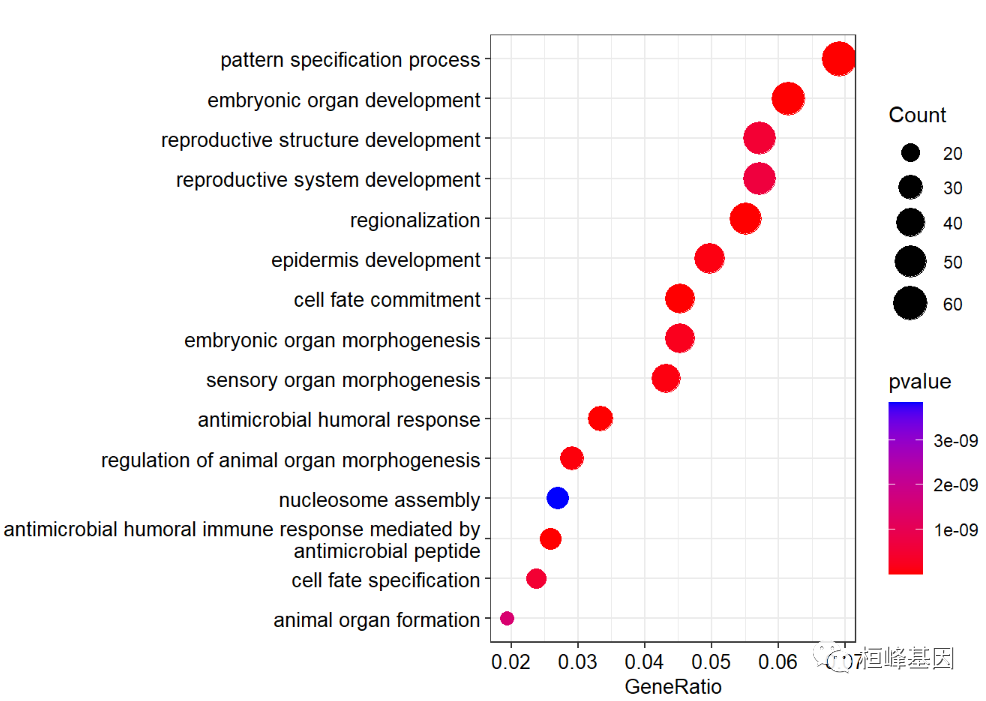
Because the description fonts of GO coincide, we use scale_ y_ Set discrete to prevent fonts from overlapping each other, as follows:
dotplot(go,
        showCategory=15,
        font.size=10,
        color ="pvalue")+
  scale_y_discrete(labels=function(x) stringr::str_wrap(x, width=60))
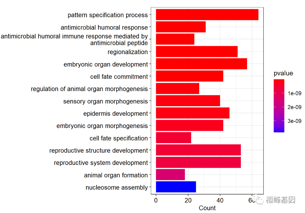
Draw a histogram as follows:
barplot(go,
        showCategory=15,
        font.size=10,
        color ="pvalue")+
  scale_y_discrete(labels=function(x) stringr::str_wrap(x, width=60))


## Scale for 'y' is already present. Adding another scale for 'y', which
## will replace the existing scale.
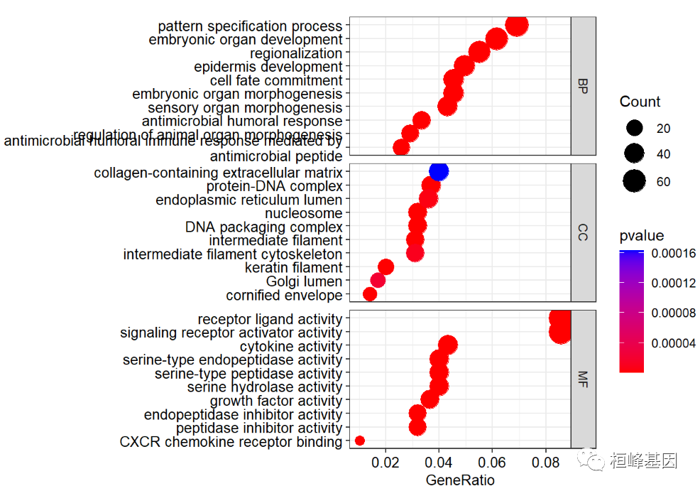
We can use split = "ONTOLOGY" method to draw three biological classifications separately on a map, as follows:
dotplot(go,showCategory=10,
        font.size=10,
        split="ONTOLOGY",
        color ="pvalue")+
  facet_grid(ONTOLOGY~.,scale="free")+
  scale_y_discrete(labels=function(x) str_wrap(x, width=60))


## Scale for 'y' is already present. Adding another scale for 'y', which
## will replace the existing scale.
We can use split = "ONTOLOGY" method to draw three biological classifications separately on a map, as follows:
barplot(go,showCategory=10,
        font.size=10,
        split="ONTOLOGY",
        color ="pvalue")+
  facet_grid(ONTOLOGY~.,scale="free")+
  scale_y_discrete(labels=function(x) str_wrap(x, width=60))


## Scale for 'y' is already present. Adding another scale for 'y', which
## will replace the existing scale.
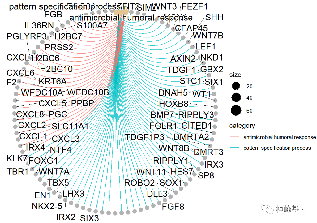
Draw the network diagram of gene concept and the network diagram of the relationship between GO term and differential gene gene gene concept network to show and explain the corresponding relationship between genes and enriched GO terms: the gray points in the figure represent genes and the Yellow points represent enriched GO terms; If a gene is located under a go term, connect the gene with go; The size of the Yellow node corresponds to the number of genes enriched, and the GO terms enriched by top2 are as follows:
cnetplot(go,showCategory=2,circular=TRUE,colorEdge=TRUE)


## Warning: ggrepel: 14 unlabeled data points (too many overlaps). Consider
## increasing max.overlaps
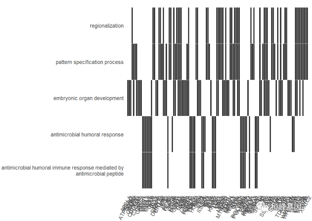
The heat map shows which genes are enriched to which go terms, as follows:
heatplot(go,showCategory=5)+
 scale_y_discrete(labels=function(x) stringr::str_wrap(x, width=60))

## Scale for 'y' is already present. Adding another scale for 'y', which
## will replace the existing scale.
The software is installed and loaded as follows:
if(!require(ggnewscale)){
  install.packages("ggnewscale")
}
library(enrichplot)
library(ggnewscale)
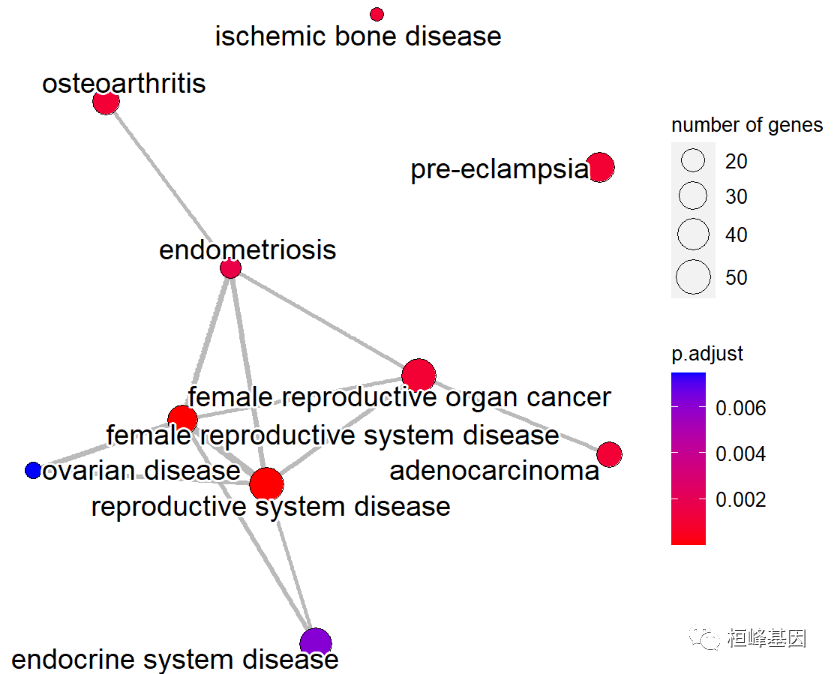
You can choose a more beautiful network diagram as follows:
ed = enrichDO(eg$ENTREZID, pvalueCutoff=0.05)
met <- pairwise_termsim(ed)
emapplot(met,showCategory = 10)
Let's look at several ways to draw the tree diagram of GO term. First, we annotate go with BP type, as follows:
###########BP classification display
BP <- enrichGO(eg$SYMBOL,
               OrgDb = org.Hs.eg.db,
               ont='BP',
               keyType = "SYMBOL",
               pAdjustMethod = 'BH',
               pvalueCutoff = 0.01,
               qvalueCutoff = 0.05,
               #keyType = 'ENTREZID'
)
dim(BP)


## [1] 193   9
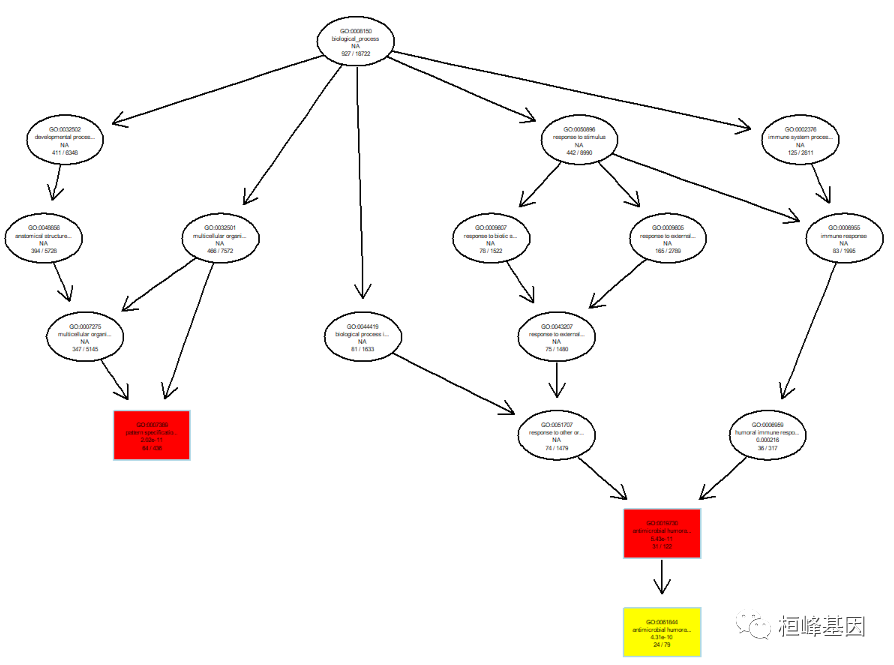
GO DAG graph, a directed acyclic graph, calls the topGO software package. We find that the font on this graph is very small, and we need to modify it ourselves later, as follows:
plotGOgraph(BP, sigForAll =FALSE,firstSigNodes = 3)
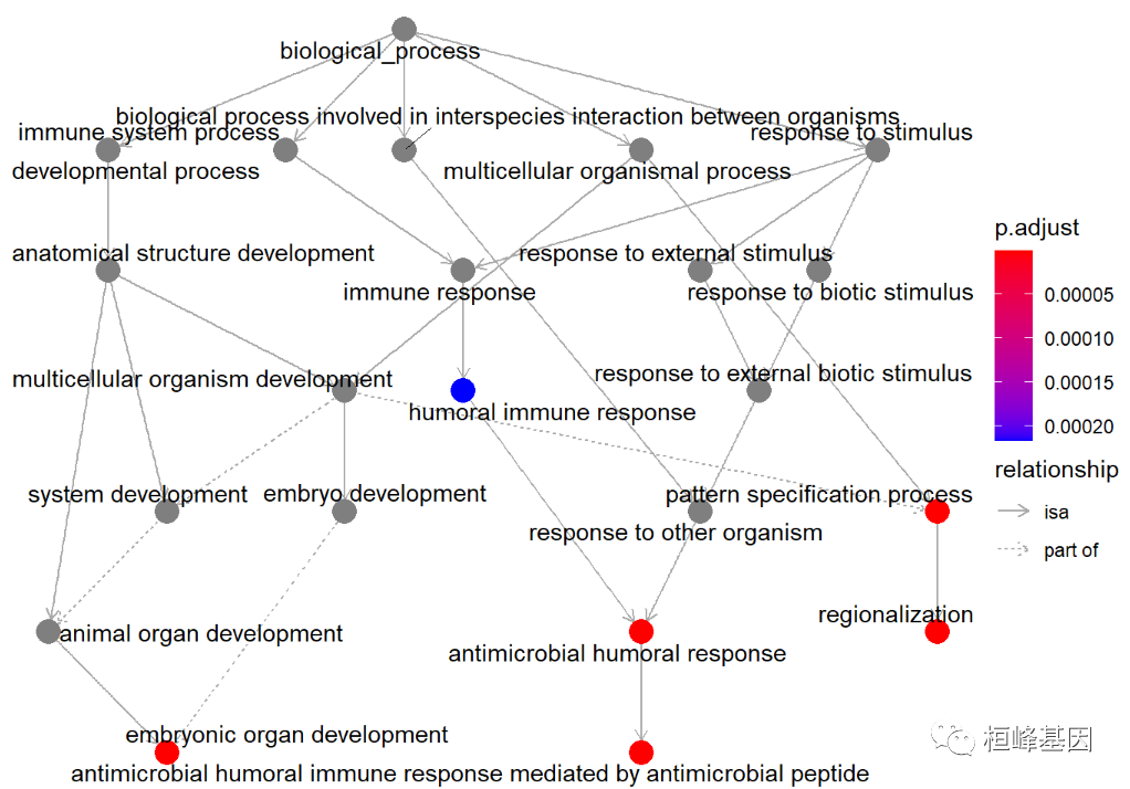
Use the enrichPlot software package to draw the diagram, as follows:
goplot(BP, showCategory = 5)
The results of GO annotation are displayed in various forms, and I feel that the summary has been very comprehensive. If there is anything I can't take into account, you can point out that I'll modify it and select the model based on my own article.
Pay attention to the official account, update every day, sweep the code into groups and communicate with each other without stopping, immediately release the video version, pay attention to me, your best choice!

Huanfeng gene
Bioinformatics analysis, SCI article writing and bioinformatics basic knowledge learning: R language learning, perl basic programming, linux system commands, Python meet you better
46 original content
official account
References:
-
Ashburner M, Ball CA, Blake JA, et al. Gene ontology: tool for the unification of biology. The Gene Ontology Consortium. Nat Genet. 2000;25(1):25-29.
-
Yu G, Wang L, Han Y and He Q*. clusterProfiler: an R package for comparing biological themes among gene clusters. OMICS: A Journal of Integrative Biology. 2012, 16(5):284-287.