RNN and its code flow

This paper focuses on the whole process of RNN rather than the derivation process of BP

What is RNN

• Recurrent Neural Network

• Cyclic neural network

Why do you need RNN?

Ordinary neural networks can only deal with one input separately, and the former input has nothing to do with the latter input. However, some tasks need to be able to better process sequence information, that is, the previous input is related to the subsequent input

**For example, when we understand the meaning of a sentence, it is not enough to understand each word of the sentence in isolation. We need to deal with the whole sequence of these words** When we process video, we can not only analyze each frame separately, but also analyze the whole sequence connected by these frames.

For example: take simple part of speech tagging as an example

• Enter "I eat apples"
• Output as "I / n eat / v apple / n"
• Obviously, the probability that "apple" after "eat" is a noun is greater than a verb
• Conclusion: the information of a location will be affected by its previous information
• RNN is a neural network that can store the previous time step information

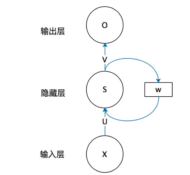
Basic framework of RNN (cyclic neural network)

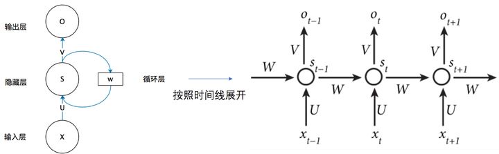
It should be noted in the figure below that the self circulation model on the left is the real RNN structure. The model on the right is just that we expand the structure of RNN in time steps for easy understanding

• The information of the upper layer is retained through the hidden layer, which will be transmitted to the next time step
• Look at the right half of the picture above
  • x t x_t xt ， yes t t Input of t time steps, s t s_t st ， yes t t The hidden information retained in t time steps, that is, the information of the previous time step, which will be transferred to the second time step t + 1 t+1 t+1 time steps are passed on.
  • O t O_t Ot ， is the second t t Output of t time steps
  • W , U , V W , U , V W. U and V are weight matrices
  • O t = g ( V ⋅ S t ) O_{t}=g\left(V \cdot S_{t}\right) Ot​=g(V⋅St​)
  • S t = f ( U ⋅ X t + W ⋅ S t − 1 ) S_{t}=f\left(U \cdot X_{t}+W \cdot S_{t-1}\right) St​=f(U⋅Xt​+W⋅St−1​)
• Now go back to the left
  • The time step is actually the first, second and second time of the model work t t t times.
  • There is an input for each model work x x x. And the information left by the previous work, that is, the hidden layer s s s. Then the model passes the formula S = f ( U ⋅ X + W ⋅ S ) S=f\left(U \cdot X+W \cdot S\right) S=f(U ⋅ X+W ⋅ S) updates the hidden layer information, that is, add the information entered this time to the past information, and then pass it to the next layer
  • The hidden layer information of the current layer combines the previous information and the information input this time, so the output can be determined. We use O = g ( V ⋅ S ) O=g\left(V \cdot S\right) O=g(V ⋅ S) get the output of the current model

Test the effect of the model (use the model to generate the sampling function of the sentence)

• sample function

  def sample(h, seed_ix, n): # Create an index sequence
    # h is the state of the hidden layer, that is, the information left by the previous time step
    #vocab_size is the number of letters that are not repeated. Here we vectorize the letters. Each letter corresponds to a position in x. if the position is 1, it means that the letter appears. If it is 0, it does not appear
    x = np.zeros((vocab_size, 1))
    x[seed_ix] = 1 # seed_ix is a number
    print("seed_ix:%s" % seed_ix)
    ixes = []
    for t in range(n): # A total of n index es are taken out
      h = np.tanh(np.dot(Wxh, x) + np.dot(Whh, h) + bh)
      y = np.dot(Why, h) + by
      p = np.exp(y) / np.sum(np.exp(y))
      ix = np.random.choice(range(vocab_size), p=p.ravel())
      x = np.zeros((vocab_size, 1))
      x[ix] = 1
      ixes.append(ix)
    return ixes
  

  • Function: input the index of a letter, use the current RNN model to create the whole sentence according to the letter, and then return to the index list corresponding to the letter in the sentence

  • input

    • h is the state of the hidden layer, that is, the information left by the previous time step
    • seed_ix is an index, that is, the index corresponding to the letter we want to enter
    • n: Sentence length (number of alphabetic indexes to be generated)

  • Analysis 1

      x = np.zeros((vocab_size, 1))
      x[seed_ix] = 1 # Get the coding vector of the corresponding letter of the access index
      print("seed_ix:%s" % seed_ix)
      ixes = []
    

    • vocab_size is the number of letters that are not repeated. Here we vectorize the letters. Each letter corresponds to a position in x. if the position is 1, it means that the letter appears. If it is 0, it does not appear
    • It's one hot coding

  • Analysis 2

     for t in range(n): # A total of n index es are taken out
        h = np.tanh(np.dot(Wxh, x) + np.dot(Whh, h) + bh)
        y = np.dot(Why, h) + by
        p = np.exp(y) / np.sum(np.exp(y))
        ix = np.random.choice(range(vocab_size), p=p.ravel())
        x = np.zeros((vocab_size, 1))
        x[ix] = 1
        ixes.append(ix) #Put in the ixes list
    

    • h is the hidden layer state

    • Note: the h corresponding to each t is different, and the h here is updated

    • y: Score vector. Each score is the score of the letter corresponding to the index of the score

    • p: Using softmax, the score is transformed into probability

    • ix: take out an index according to the probability in p

    • Reset the encoding vector x for the next time step

    • Is to achieve the following process

      

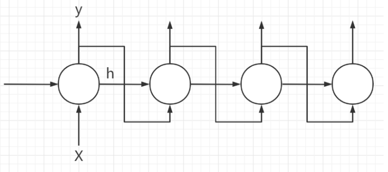
lossFun (loss function)

• lossFun

  • The process is introduced in detail, and the gradient calculation in BP process is not introduced in detail

  def lossFun(inputs, targets, hprev):
    """
    inputs,targets are both list of integers.
    hprev is Hx1 array of initial hidden state
    returns the loss, gradients on model parameters, and last hidden state
    """
    xs, hs, ys, ps = {}, {}, {}, {}
    hs[-1] = np.copy(hprev)
    loss = 0
    # forward pass
    for t in range(len(inputs)): # inputs are all array < int > types
      # Encode elements as vectors
      xs[t] = np.zeros((vocab_size,1)) # Initialize to 0 vector
      # print("input: %s" % inputs[t])
      # print("type: %s" % type(inputs[t]))
      xs[t][inputs[t]] = 1
      hs[t] = np.tanh(np.dot(Wxh, xs[t]) + np.dot(Whh, hs[t-1]) + bh) # hidden state
      ys[t] = np.dot(Why, hs[t]) + by # unnormalized log probabilities for next chars
      ps[t] = np.exp(ys[t]) / np.sum(np.exp(ys[t])) # probabilities for next chars
      loss += -np.log(ps[t][targets[t],0]) # softmax (cross-entropy loss)
         
      
    # BP process, calculating gradient
    dWxh, dWhh, dWhy = np.zeros_like(Wxh), np.zeros_like(Whh), np.zeros_like(Why)
    dbh, dby = np.zeros_like(bh), np.zeros_like(by)
    dhnext = np.zeros_like(hs[0])
    for t in reversed(range(len(inputs))):
      dy = np.copy(ps[t])
      dy[targets[t]] -= 1 # backprop into y. see http://cs231n.github.io/neural-networks-case-study/#grad if confused here
      dWhy += np.dot(dy, hs[t].T)
      dby += dy
      dh = np.dot(Why.T, dy) + dhnext # backprop into h
      dhraw = (1 - hs[t] * hs[t]) * dh # backprop through tanh nonlinearity
      dbh += dhraw
      dWxh += np.dot(dhraw, xs[t].T)
      dWhh += np.dot(dhraw, hs[t-1].T)
      dhnext = np.dot(Whh.T, dhraw)
    for dparam in [dWxh, dWhh, dWhy, dbh, dby]:
      np.clip(dparam, -5, 5, out=dparam) # clip to mitigate exploding gradients
    return loss, dWxh, dWhh, dWhy, dbh, dby, hs[len(inputs)-1]
  

  • Input a string of characters to train the model and return the gradient of loss and various parameters

  • Input:

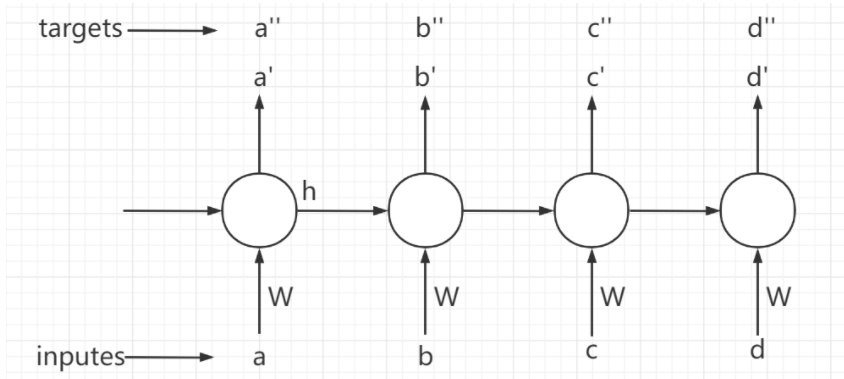
    • inputs: input of model training data, i.e. [a, B, C, D] shown in the figure above
    • targets: the correct result that the model should produce for inputs, that is, [a ', b', c ', d'] as shown in the figure above
    • hprev: vector of H-by-1. Represents the initial state of the hidden layer of each neuron in the current time step

  • Analysis 1

      xs, hs, ys, ps = {}, {}, {}, {}
      hs[-1] = np.copy(hprev)
      loss = 0
    

    • For each character input, it trains models with different time steps. eg:
      • inputs = [a , b , c , d]
      • a trains the model at t = 1
      • b trains the model at t = 2
      • c trains the model at t = 3
      • d trains the model at t = 4
    • This code is just initialization

  • Analysis 2

    for t in range(len(inputs)): #inputs are all array < int > types
        # Encode elements as vectors
        xs[t] = np.zeros((vocab_size,1)) # Initialize to 0 vector
        xs[t][inputs[t]] = 1
        hs[t] = np.tanh(np.dot(Wxh, xs[t]) + np.dot(Whh, hs[t-1]) + bh) # hidden state
        ys[t] = np.dot(Why, hs[t]) + by # unnormalized log probabilities for next chars
        ps[t] = np.exp(ys[t]) / np.sum(np.exp(ys[t])) # probabilities for next chars
        loss += -np.log(ps[t][targets[t],0]) # The score of the correct result, the greater the score, the smaller the loss
    

    • Note: when traversing the inputs, the index is used as the time step. hs[t-1] is always changing, and the information of the previous time step is stored
    • Traverse each input character
    • Establish one hot encoding for a character
    • Calculates the hidden state of the current time step
    • Note: the parameter matrix of each time step is the same, which is essentially the training of a model, but the input characters are different from the hidden state
    • Calculate the output of different time steps (fractional vector), that is, the output corresponding to different characters
    • Transform fractional vector into probability vector using softmax
    • Calculate the loss generated by each character

• main function

  • In the process of one training, the parameter matrix of the model in different time steps is the same, because in essence, one model is trained in time
  • One SEQ at a time_ Long data training model
  • The detailed process is marked in the notes

  n, p = 0, 0
  mWxh, mWhh, mWhy = np.zeros_like(Wxh), np.zeros_like(Whh), np.zeros_like(Why)
  mbh, mby = np.zeros_like(bh), np.zeros_like(by) # memory variables for Adagrad
  smooth_loss = -np.log(1.0/vocab_size)*seq_length # loss at iteration 0
  
  while True:
    if p + seq_length + 1 >= len(data) or n == 0: # It is initialized at the beginning or at the end
      hprev = np.zeros((hidden_size,1)) # Reset hidden layer state
      p = 0 # Point to the first of the input data
  
    # targets is a word pushed back by inputs
    inputs = [char_to_ix[ch] for ch in data[p:p+seq_length]] # A list storing index
    targets = [char_to_ix[ch] for ch in data[p+1:p+seq_length+1]] # A list storing index
  
    # This sampling is just to try the effect of the model, sampling every 100 times
    if n % 100 == 0:
      sample_ix = sample(hprev, inputs[0], 200) # Sampling to obtain the index sequence of the sampled words
      txt = ''.join(ix_to_char[ix] for ix in sample_ix) # Output these words through the obtained index sequence
      print ('----\n %s \n----' % (txt, ))
  
    # Using seq_ For the data of length, the loss and gradient of the model are calculated once
    loss, dWxh, dWhh, dWhy, dbh, dby, hprev = lossFun(inputs, targets, hprev) # Get Loss and gradient
    smooth_loss = smooth_loss * 0.999 + loss * 0.001
    if n % 100 == 0: print ('iter %d, loss: %f' % (n, smooth_loss)) # 100 times one output
    
    # Parameter update
    for param, dparam, mem in zip([Wxh, Whh, Why, bh, by], 
                                  [dWxh, dWhh, dWhy, dbh, dby], 
                                  [mWxh, mWhh, mWhy, mbh, mby]):
      mem += dparam * dparam # The corresponding position point of dparam multiplied by mem is the sum of squares of the front gradient
      
      #The more you go to the back, the less you learn
      param += -learning_rate * dparam / np.sqrt(mem + 1e-8) # adagrad update
  
    p += seq_length # p points to the next SEQ_ Start of length
    n += 1 # iteration counter