2021SC@SDUSC

(12) lvi-sam source code read 10 - visual_loop Reading 3 + ORB learning

visual_loop

DUtils Folder

DException

Define exception information

Timestamp

//Member variables
    /// Seconds
    unsigned long m_secs;	// seconds
    /// Microseconds
    unsigned long m_usecs;	// microseconds

//Main methods
 setTime //Set time stamp
 getTime //Get between timestamps

Random

Generating Random Numbers with Gauss Distribution

/**
 * Returns a random number in the range [0..1]
 * @return random T number in [0..1]
 */
template <class T>
static T RandomValue(){
	return (T)rand()/(T)RAND_MAX;
}

/**
 * Returns a random number in the range [min..max]
 * @param min
 * @param max
 * @return random T number in [min..max]
 */
template <class T>
static T RandomValue(T min, T max){
    return Random::RandomValue<T>() * (max - min) + min;
}

/** 
 * Returns a random number from a gaussian distribution
 * @param mean
 * @param sigma standard deviation
 */
template <class T>
//Given mathematical expectations and standard deviations
static T RandomGaussianValue(T mean, T sigma)
{
    // Box-Muller transformation
    T x1, x2, w, y1;

    do {
      //2.0 is double
      x1 = (T)2. * RandomValue<T>() - (T)1.;
      x2 = (T)2. * RandomValue<T>() - (T)1.;
      w = x1 * x1 + x2 * x2;
    } while ( w >= (T)1. || w == (T)0. );

    w = sqrt( ((T)-2.0 * log( w ) ) / w );
    y1 = x1 * w;

    return( mean + y1 * sigma );
}

Generate random numbers with Gaussian or any other distribution https://www.cnblogs.com/mightycode/p/8370616.html

DVision Folder

DVision.h

DVision itself is an open source library with corresponding dependencies and libraries in python and c++, and a collection of classes with computer vision capabilities.

This project should be part of an embedded open source library.

There is a namespace DVision defined inside the file, but there is no content inside (should be deleted from the namespace in the original library)

BRIEF

BRIEF is a descriptor in ORB feature points. In order to get a better understanding of BRIEF, I first learned the feature points of the seventh lecture in SLAM14, which is also mainly explained with ORB as an example.

The purpose of this file is to find the BRIEF descriptor of each point for a given image and key points in the image.

//Member variables
/// Descriptor length in bits
int m_bit_length;

/// Patch size
int m_patch_size;

/// Type of pairs
Type m_type;

/// Coordinates of test points relative to the center of the patch
std::vector<int> m_x1, m_x2;
std::vector<int> m_y1, m_y2;

//Key Functions

//Generate the location of selected random points, stored in m_ In vector s of
void BRIEF::generateTestPoints()

//Returns a brief descriptor of a given key point in a given image
void BRIEF::compute(const cv::Mat &image,  //image
    const std::vector<cv::KeyPoint> &points,   //
    vector<bitset> &descriptors,  //descriptor
    bool treat_image) const
{
  const float sigma = 2.f;
  const cv::Size ksize(9, 9);
  
  cv::Mat im;
  if(treat_image)
  {
    cv::Mat aux;
    if(image.depth() == 3)
    {
      cv::cvtColor(image, aux, CV_RGB2GRAY);
    }
    else
    {
      aux = image;
    }

    cv::GaussianBlur(aux, im, ksize, sigma, sigma);
    
  }
  else
  {
    im = image;
  }
  
  assert(im.type() == CV_8UC1);
  assert(im.isContinuous());
  
  // use im now
  const int W = im.cols;
  const int H = im.rows;
  
  descriptors.resize(points.size());
  //The bitset of C++ is an array-like structure in the bitset header file, where each element can only be 0 or 1, and each element only uses 1 bit of space.
  std::vector<bitset>::iterator dit; // Store each feature

  std::vector<cv::KeyPoint>::const_iterator kit;
  
  int x1, y1, x2, y2;
  
  dit = descriptors.begin();
  for(kit = points.begin(); kit != points.end(); ++kit, ++dit)
  {
    dit->resize(m_bit_length);
    dit->reset();

    for(unsigned int i = 0; i < m_x1.size(); ++i)
    {
      x1 = (int)(kit->pt.x + m_x1[i]);
      y1 = (int)(kit->pt.y + m_y1[i]);
      x2 = (int)(kit->pt.x + m_x2[i]);
      y2 = (int)(kit->pt.y + m_y2[i]);
      
      if(x1 >= 0 && x1 < W && y1 >= 0 && y1 < H 
        && x2 >= 0 && x2 < W && y2 >= 0 && y2 < H)
      {
        //Determine the size of the two selected pixel points
        if( im.ptr<unsigned char>(y1)[x1] < im.ptr<unsigned char>(y2)[x2] )
        {
          //Set the ith bit of dit to 1
          dit->set(i);
        }        
      } // if (x,y)_1 and (x,y)_2 are in the image
            
    } // for each (x,y)
  } // for each keypoint
}

bitset https://www.cnblogs.com/magisk/p/8809922.html

Pre-learning

Eigenvalue method

The front end based on feature points has long been the mainstream method for visual milemeters.

1.1 Feature Point

The core issue of a visual milemeter is how to estimate camera motion from images. It is convenient to select representative points from the image that will remain unchanged when the camera's perspective changes. In classical SLAM problems, we call these points signposts. In visual SLAM problems, landmarks refer to image features.

Feature: is another digital representation of image information.

It is not possible to determine which points are the same by the gray value characteristics of the pixels alone (gray values are heavily affected by illumination, distortion, and object materials).

Feature points: Some special things in the image.

An intuitive way to extract feature points is to identify corners between different images and determine their corresponding relationships. In this way, corners are the so-called characteristics.

Corner extraction algorithm: Harris Corner, FAST Corner, GFTT Corner...

But simple corners don't satisfy many requirements (eg: Where it looks like a corner from a distance, it may no longer appear as a corner when the camera is close enough). For this reason, there are many more stable local image features, such as SIFT, SURF, ORB, and so on.

These artificially designed features can have the following properties:

• Repeatability: The same feature points can be found in different images
• Distinctivity: Different features have different representations
• Efficiency: In the same image, the number of feature points should be much smaller than the number of pixels
• Locality: Features are associated with only a small area of the image

Feature Points: By Key-Point and descriptor

• Key Points: refers to the position of the feature in the image. Some feature points also have orientation, size and other information.
• Descriptor: Usually a vector describing information about pixels around a key point in an artificially designed way. Descriptors are designed according to the principle that features with similar appearance should have similar descriptors. Therefore, as long as the descriptors of the two feature points are close in vector space, we can assume that they are the same feature points.

ORB (Oriented FAST and Rotated BRIEF) feature is a representative real-time image feature at present. The non-directional problem in FAST detectors was improved by using the fast binary descriptor BRIEF (Binary Robust Independenct Elementary Feature). ORB maintains the rotation and scale invariance of the feature subunits, and improves the speed significantly. It is a good choice for SLAM with high real-time requirements.

1.2 ORB characteristics

ORB features consist of key points and descriptors. Its key point, called Oriented FAST, is an improved FAST corner point. Its descriptor is called BRIEF. Extracting ORB features is divided into two steps:

1. FAST Corner Extraction: Find the corners in the image. Compared with the original FAST, the main direction of the feature points is calculated in ORB, which adds the rotation invariant feature to the subsequent BRIEF descriptors.
2. BRIEF descriptor: Describes the image area around the feature point extracted in the previous step. ORB and BRIEF have made some improvements, mainly referring to the use of previously calculated direction information in BRIEF.

FAST Key Points

FAST is a corner point that detects where the local pixel gray level changes significantly. Idea: If a pixel is very different from its neighbors (too bright or too dark), it is more likely to be a corner point.

Detection process:

1. Pixel p is selected in the image, assuming brightness is Ip.
2. Set a threshold T (less than 20% of Ip).
3. With pixel p as the center, select 16 pixel points on a circle with radius 3
4. If N consecutive points on the selected circle are brighter than Ip+T or less than Ip-T, then pixel p can be considered as a feature point (N usually takes 12, FAST-12).
5. Cycle through the four steps above to perform the same operation for each pixel

• In the FAST-12 algorithm, to be more efficient, a pilot operation can be added to quickly exclude the vast majority of pixels that are not corner points: for each pixel, directly check the brightness of 1,5913 pixels on the neighborhood circle, and only if at least three of these four points meet the criteria, the current pixel may be a corner point
• The original FAST corners are prone to corner clumping, so after the first detection, non-maximum suppression is also needed to keep only the corner points that respond to the maximum values in a certain area to avoid the problem of corner set.

Advantages and disadvantages of FAST corner points: Just compare the brightness differences between pixels, so it's fast; However, they are not reproducible and unevenly distributed. FAST corner does not have direction information. Because a circle with a fixed radius of 3 has a scale problem.

For the disadvantage of FAST corner having no directionality and scale, ORB adds a description of scale and rotation.

Scale invariance: is achieved by building image pyramids and detecting corner points on each layer of the pyramid

• The pyramid base is the original image, and each layer up, the image is scaled at a fixed magnification, resulting in images of different resolutions. Smaller images can be seen as scenes from a distance. In the feature matching algorithm, we can match images on different layers to achieve scale invariance.
• eg: If the camera goes back, we should be able to find a match above the previous image pyramid and below the next image pyramid

Rotation: achieved by gray scale centroid method

• Calculate the gray centroid of the image near the feature point.

• Centroid is the center with image gray value as weight

• Steps:

  

  

This improved FAST is called Oriented FAST.

BRIEF descriptor

After extracting the Oriented FAST corner points, we calculate their descriptors for each of them. ORB uses the improved BRIEF feature description.

BRIEF is a binary descriptor whose description vector consists of 0/1, where 0 and 1 encode the size relationship of two random pixels (e.g., p and q) near a critical point: if p is larger than q, take 1; The opposite is 0. If we randomly delete 128 such sets of p and q, we will end up with a 128-dimensional vector of 0 and 1.

BRIEF uses a random selection comparison, which is very fast and easy to store due to binary representation, and is suitable for real-time image matching.

The original BRIEF descriptors do not have rotation invariance, so they are easily lost when the image is rotated. ORB calculates the direction of key points in the FAST feature point extraction stage, so the steer BRIEF feature after rotation can be calculated to make the descriptor of ORB have good rotation invariance.

1.3 Feature Matching

Feature matching solves the data association problem in SLAM problems.

Due to the local characteristics of image features, mismatching is widespread and has not been effectively solved for a long time. It has become a major bottleneck in the performance constraints of visual SLAM. Part of the reason is that there are often a lot of duplicate textures in the scene, which makes the feature descriptions very similar. In this case, it is very difficult to resolve mismatches only by using local features.

Violent matching is the easiest way to match

For binary descriptors, the Hamming distance can be used as a measure - the Hamming distance between two binary strings refers to the number of different digits.

The FLANN (Fast Approximate Nearest Neighbor) algorithm is suitable for situations where the number of matching points is very large.

Nonmaximum Suppression

NMS (non maximum suppression), Chinese name non maximum suppression, is widely used in many computer vision tasks, such as edge detection, target detection, and so on.

NMS, as its name implies, suppresses elements that are not maximums and can be interpreted as local maximum searches. This locally represents a neighborhood with two variable parameters: the dimension of the neighborhood and the size of the neighborhood. The window with the highest score for extraction in target detection is discussed here. For example, in pedestrian detection, the sliding window extracts the features, and each window gets a score after being classified and identified by the classifier. However, sliding windows can cause many windows to contain or mostly cross other windows. NMS is then used to select those neighborhoods with the highest score (the most likely pedestrian) and to suppress those windows with the lowest score.

NMS plays an important role in computer vision, such as video target tracking, data mining, 3D reconstruction, target recognition and texture analysis.

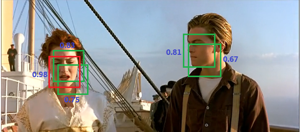
For example, in the following figure, because of the sliding window, the same person may have several boxes (each with a classifier score)

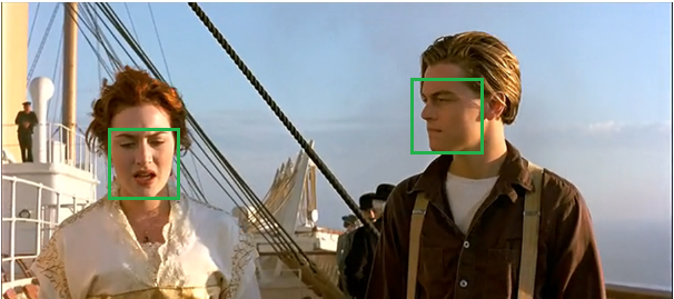
Our goal is to keep only one of the best boxes:

We then use non-maximum suppression to suppress redundant boxes: suppression is an iteration-traversal-elimination process.

**(1)** Sort the scores of all boxes, and select the highest score and its corresponding box:

**(2)**Walk through the remaining boxes and delete them if the overlap area (IOU) with the current highest box is greater than a certain threshold.

**(3)** Repeat the process by continuing to select the box with the highest score from which you have never processed.

NSM-Nonmaximum Suppression https://blog.csdn.net/shuzfan/article/details/52711706

https://www.cnblogs.com/makefile/p/nms.html

FLANN algorithm

FLANN libraries can be called directly in opencv.

FLANN is short for Fast_Library_for_Approximate_Nearest_Neighbors. It is a collection of nearest neighbor search algorithms for large datasets and high-dimensional features that have been optimized. It works better against large datasets than BFMatcher.

https://blog.csdn.net/jinxueliu31/article/details/37768995

https://blog.csdn.net/Bluenapa/article/details/88371512

http://www.whudj.cn/?p=920