1. The author may divide the scanner data set into training set and test set and process them into. pickle files.
2. In the process of code running, the author read out the x, y, z coordinates of 1201 scenes in the training set and 312 scenes in the test set from the. pickle file.

3. Consider saving the point to a. txt file and visualizing it with cloudcompare.
2 -- floor
Save training data to txt file separately:
TRAIN_DATASET = scannet_dataset.ScannetDataset(root=DATA_PATH, npoints=NUM_POINT, split='train')
for
 i in range(len(TRAIN_DATASET.scene_points_list)):
    filename=''.join(["TRAIN_DATASET_",str(i+1),'.txt'])
    np.savetxt(filename, TRAIN_DATASET.scene_points_list[i],fmt="%.8f", delimiter=',')
Save the label of training data to the txt file separately:
for i in range(len(TRAIN_DATASET.semantic_labels_list)):
    filename=''.join(["data/train_dataset/train_label_",str(i+1),'.txt'])
    np.savetxt(filename, TRAIN_DATASET.semantic_labels_list[i],fmt="%d", delimiter=',')
Save the test data to the txt file separately:
TEST_DATASET = scannet_dataset.ScannetDataset(root=DATA_PATH, npoints=NUM_POINT, split='test')
for i in range(len(TEST_DATASET.scene_points_list)):
    filename=''.join(["data/test_dataset/test_",str(i+1),'.txt'])
    np.savetxt(filename, TEST_DATASET.scene_points_list[i],fmt="%.8f", delimiter=',')
Save the label of test data to the txt file separately:
for i in range(len(TEST_DATASET.semantic_labels_list)): filename=''.join(["data/test_dataset/test_",str(i+1),'.txt']) np.savetxt(filename, TEST_DATASET.semantic_labels_list[i],fmt="%.8f", delimiter=',')
Put the training set and its corresponding tags together:
traindata_and_label=np.column_stack((TRAIN_DATASET.scene_points_list, TRAIN_DATASET.semantic_labels_list))#np.column_stack Combining two matrices
    filename=''.join(["data/train_dataset/train_data_and_label_",str(1),'.txt'])
    np.savetxt(filename, traindata_and_label,fmt="%.8f,%.8f,%.8f,%d", delimiter=',')
Put the test set and its corresponding labels together:
traindata_and_label=np.column_stack((TEST_DATASET.scene_points_list, TEST_DATASET.semantic_labels_list))#np.column_stack Combining two matrices
    filename=''.join(["data/test_dataset/test_data_and_label_",str(1),'.txt'])
    np.savetxt(filename, testdata_and_label,fmt="%.8f,%.8f,%.8f,%d", delimiter=',')
4.
def __getitem__(self, index):
        point_set = self.scene_points_list[index]
        semantic_seg = self.semantic_labels_list[index].astype(np.int32)
        coordmax = np.max(point_set,axis=0)
        coordmin = np.min(point_set,axis=0)
        smpmin = np.maximum(coordmax-[1.5,1.5,3.0], coordmin) #(1)
        smpmin[2] = coordmin[2]
        smpsz = np.minimum(coordmax-smpmin,[1.5,1.5,3.0])
        smpsz[2] = coordmax[2]-coordmin[2]
        isvalid = False
        #global sample_weight  # 2019.11.4
        sample_weight=0  # 2019.11.4
#(1) For scene sampling, the voxel size is 1.5 * 1.5 * 3. Some scenes may not have a height of 3m, so the voxel height is based on the actual minimum bounding box height of the scene.
Original text:
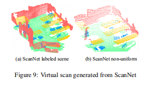
B.2 virtual scan generation
In this section, we describe how to generate a labeled virtual scan with non-uniform sampling density from a scanned network scene. For each scene in ScanNet, we set the camera position to 1.5m higher than the plane centroid, and rotate the camera direction evenly in 8 directions in the horizontal plane. In each direction, we use an image plane with a size of 100px and project light from each pixel to the scene. This gives a method of selecting visible points in the scene. Then, we can generate eight virtual scans similar to each test scenario, and an example is shown in Figure 9. Note that point samples are more dense near the camera.
B.4 scanning network experiment details
In order to generate training data from the ScanNet scene, we sample a cube as large as 1.5m × 1.5m × 3m from the initial scene, and then keep the cube, where ≥ 2% of voxels are occupied, and ≥ 70% of the surface voxels have effective labeling (this is the same as the setting in [5]). We sample such a training cube in flight and rotate it randomly along the top right axis. Enhancement points are added to the point set to form a fixed cardinality (8192 in this case). During the test, we also split the test scene into smaller cubes, and first get the label prediction of each point in the cube, and then merge the label prediction from all cubes in the same scene. If a point gets a different label from a different cube, we will have a majority vote to get the final point label prediction.
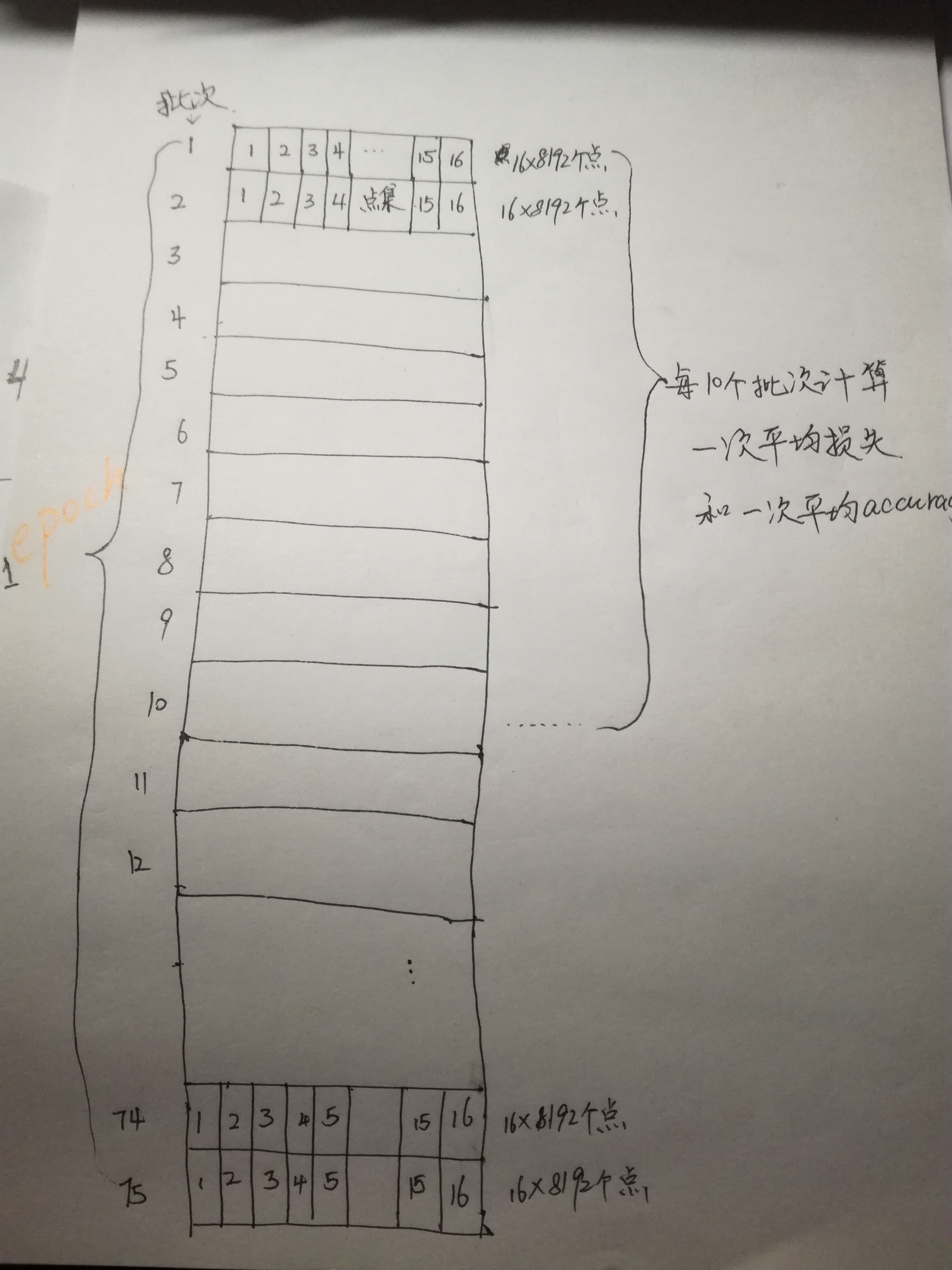
10 --- 10 batches, each batch has 16 sets of scenic spots, each point set has 8192 points
20 --- 20 batches, each batch has 16 sets of scenic spots, each set has 8192 points
1 BatchSize=16 or 32 data sets
75----Total BatchSize, 1201 datasets. If 16 datasets are used as 1 batch, 1201//16=75 can be divided into 75 batches.
mean loss
accuracy
Training process:
1.
TRAIN_DATASET = scannet_dataset.ScannetDataset(root=DATA_PATH, npoints=NUM_POINT, split='train') #a
TEST_DATASET = scannet_dataset.ScannetDataset(root=DATA_PATH, npoints=NUM_POINT, split='test') #b
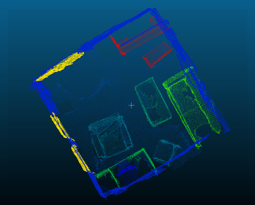
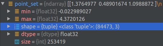
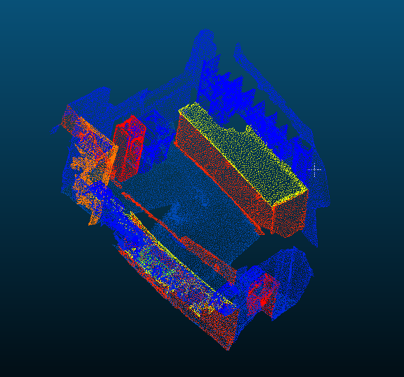
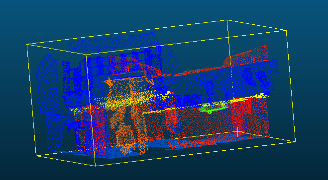
a. Load the training set. There are 1201 scenes in total. The number of point clouds in each scene is not fixed. One scene is as shown in the figure:
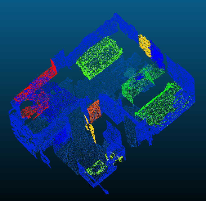
Training set: 1201 × N*3, N for points, 3 for x,y,z
Label: 1201 × N
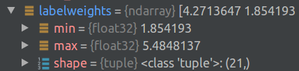
Weight: In 1201 scenes, the weight W of each category is calculated according to the proportion X of points In the total points. Calculation method: w=1 / (In (1.2+x)), (I don't know why to do this).
b. Load the test set.
Test set: 312 × N*3, N for points, 3 for x,y,z
Label: 312 × N
Weight: the weight of each category is 1
c.
TEST_DATASET_WHOLE_SCENE = scannet_dataset.ScannetDatasetWholeScene(root=DATA_PATH, npoints=NUM_POINT, split='test')
Load the test set of the whole scene, and the point cloud returned is the same as that returned by b.
2. Training model of semantic segmentation network
def get_model(point_cloud, is_training, num_class, bn_decay=None):
    """ Semantic segmentation PointNet, input is BxNx3, output Bxnum_class """
    batch_size = point_cloud.get_shape()[0].value
    num_point = point_cloud.get_shape()[1].value
    end_points = {}
    l0_xyz = point_cloud
    l0_points = None
    end_points['l0_xyz'] = l0_xyz

    # Layer 1
    l1_xyz, l1_points, l1_indices = pointnet_sa_module(l0_xyz, l0_points, npoint=1024, radius=0.1, nsample=32, mlp=[32,32,64], mlp2=None, group_all=False, is_training=is_training, bn_decay=bn_decay, scope='layer1') #a
    l2_xyz, l2_points, l2_indices = pointnet_sa_module(l1_xyz, l1_points, npoint=256, radius=0.2, nsample=32, mlp=[64,64,128], mlp2=None, group_all=False, is_training=is_training, bn_decay=bn_decay, scope='layer2') #b
    l3_xyz, l3_points, l3_indices = pointnet_sa_module(l2_xyz, l2_points, npoint=64, radius=0.4, nsample=32, mlp=[128,128,256], mlp2=None, group_all=False, is_training=is_training, bn_decay=bn_decay, scope='layer3') #c
    l4_xyz, l4_points, l4_indices = pointnet_sa_module(l3_xyz, l3_points, npoint=16, radius=0.8, nsample=32, mlp=[256,256,512], mlp2=None, group_all=False, is_training=is_training, bn_decay=bn_decay, scope='layer4') #d

    # Feature Propagation layers
    l3_points = pointnet_fp_module(l3_xyz, l4_xyz, l3_points, l4_points, [256,256], is_training, bn_decay, scope='fa_layer1')
    l2_points = pointnet_fp_module(l2_xyz, l3_xyz, l2_points, l3_points, [256,256], is_training, bn_decay, scope='fa_layer2')
    l1_points = pointnet_fp_module(l1_xyz, l2_xyz, l1_points, l2_points, [256,128], is_training, bn_decay, scope='fa_layer3')
    l0_points = pointnet_fp_module(l0_xyz, l1_xyz, l0_points, l1_points, [128,128,128], is_training, bn_decay, scope='fa_layer4')

    # FC layers
    net = tf_util.conv1d(l0_points, 128, 1, padding='VALID', bn=True, is_training=is_training, scope='fc1', bn_decay=bn_decay)
    end_points['feats'] = net
    net = tf_util.dropout(net, keep_prob=0.5, is_training=is_training, scope='dp1')
    net = tf_util.conv1d(net, num_class, 1, padding='VALID', activation_fn=None, scope='fc2')

    return net, end_points
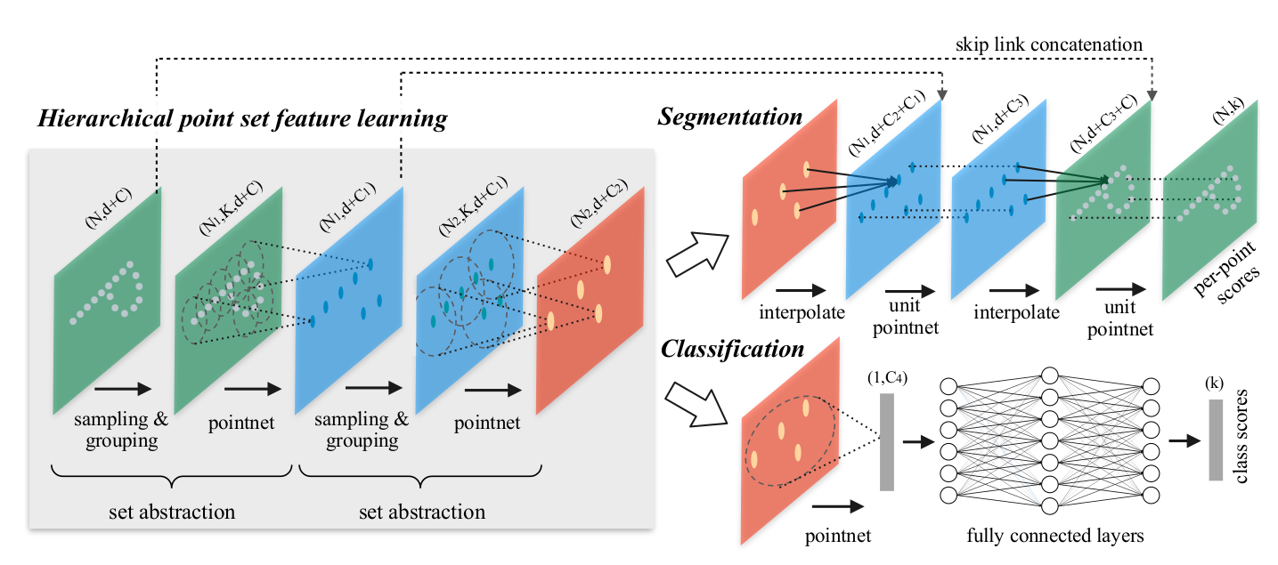
set abstraction:
a.
sampling and grouping layer
(N,d+C)=(8192,3+0)
l0_xyz, l0_points, npoint=1024, radius=0.1, nsample=32, mlp=[32,32,64]
L0 XYZ: B * n * d = 16 * 8192 * 3, enter the dimension of point cloud
l0_points: B*N*C=16*8192*0
npoint=1024, number of centroids sampled
radius=0.1, the radius of ball query. Note that this is the scale after coordinate normalization
nsample=32, the number of points in the local spherical neighborhood around each centroid
mlp=[32,32,64], use Mlp to extract the local feature vector of point cloud and the change of feature vector dimension
l0_points: < includes not only coordinates, but also features extracted after each point passes through the previous layer, so the first layer does not >
npoint = 1024: < sample layer find 512 points as the center point. This manual selection depends on experience or experiment >
radius=0.1: < the radius of the ball in the grouping layer is 0.2. Note that this is the scale after coordinate normalization >
nsample=32: < sample around each center point in the ball with a specified radius, the upper limit is 32; radius dominates >
mlp=[32,32,64]: < pointnet layer has three layers, and the change of feature dimension is 64,64128 >
grouped_xyz = group_point(xyz, idx) # (batch_size, npoint, nsample, 3) (16*1024*32*3)
    grouped_xyz -= tf.tile(tf.expand_dims(new_xyz, 2), [1,1,nsample,1]) # translation normalization   Point cloud coordinates of each region are subtracted from its centroid coordinates
new_xyz, new_points, idx, grouped_xyz = sample_and_group(npoint, radius, nsample, xyz, points, knn, use_xyz)
xyz:B*N*d=16*8192*3,Enter the dimensions of the point cloud
points: (batch_size, ndataset, channel) TF tensor (16, ndataset, channel)    (16,8192,0)
knn:false
use_xyz:use_xyz: bool, if True concat XYZ with local point features, otherwise just use point features
return:
new_xyz: (batch_size, npoint, 3) TF tensor  (16,  1024 , 3) (16,1024,3) The eigenvector is x,y,z
new_points: (batch_size, npoint, mlp[-1] or mlp2[-1]) TF tensor (16,1024,32) The eigenvector is mlp Extracted features.
idx: (batch_size, npoint, nsample) int32 -- indices for local regions (16,1024,32)
idx: is the index of points in each region (161024,32)
idx, pts_cnt = query_ball_point(radius, nsample, xyz, new_xyz)
The results of ball query are idx and PTS ﹣ CNT. Because the partition is based on radius first, the number of points in each region is uncertain (the maximum is 32), so PTS ﹣ count is count, and how many points are there in each region.
Grouped XYZ: a set of grouped points, which is a four-dimensional vector (batch size, 1024 areas, 32 points in each area, 3 coordinates for each point)
new_points: it is also the set of points after grouping, but There are features in it. If it's the first time, it's equal to grouped XYZ. You can choose to concat enate the coordinates and features during convolution
b.pointnet layer
Feature Propagation layers:
The adjacent 3-point inverse distance weighted interpolation is used.
Summary:
(1)furthest point sampling:
Each point is traversed by interval (number of sampling points), and the spatial distance between points is calculated. The point with the farthest distance is regarded as the point with the farthest distance from the current point.
For example, when the total number of points is 2048 and the sampling point is 512, traverse from the first point, calculate the distance between the first point and (1 + 512), (1 + 512 * 2), (1 + 512 * 3), regard the point with the largest distance as the point with the largest distance from the current point, and then traverse 512 times to find 512 farthest points.
(2) Gather operation: converts the Id of the point to the coordinate of the point.
(3) QueryAndGroup: connect the grouped center point coordinates and center point features.
(4) BallQuery: gather the IDs of the points whose distance from the center point is less than radius. Multiple radius can be aggregated
(5) GroupingOperation: coordinate consolidation is performed according to idx that has been grouped. (idx and N of points are passed into backward for gradient calculation when inserting points.)
(6)TreenNN: get the nearest three points around the center point of each group, and return the corresponding distance (used to calculate the weight, the weight of the far point is significant, the weight of the near point is small) and ID
(7) Three \. (advantage: in such a case, the second vector should be weighted higher. On the other hand, when the density of a local region is high, the first vector provides information of final details since it poses the ability to inspect at high resolutions recursively in lower levels.)
The convolution process can also refer to: https://blog.csdn.net/wqwqqwqw1231/article/details/90757687
3. Randomly scramble the indexes of the data sets of 1201 scenarios.
4. 1201 scene data sets are trained in batches. Each batch is divided into 16 scene data sets, i.e. numbers of one BatchSize=16, which are divided into batches with BatchSize=1201//16=75. (if it is divided into 32 scene data sets in each batch, the graphics card may not have enough memory.).
5. Before training data, load the scan_train.pickle file, which contains:
(1) 1201 scene data sets.
(2) Assume that each scene has n point clouds, and there are 1201*n point labels in the file.
(3) The initial weights of 21 categories are calculated based on the proportion of the number of point cloud labels of a certain category to all point clouds.
6. Take the point cloud data sets and corresponding point labels of the first 16 scenes in the disordered index order.
First of all, the data set of the first scene, min(x,y,z) is -0.022...max(x,y,z) is 4.37..., here we should design the preprocessing of the initial data set, I don't know how the author deals with this coordinate, generally it may be to translate the original coordinate of the data set coordinate system to its center of gravity, or to the minimum position of its bounding box (minimum corner point).
(7)
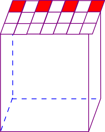
smpmin = np.maximum(coordmax-[1.5,1.5,3.0], coordmin)
Point A in the upper right corner samples inwards, the size is 1.5 * 1.5 × h, and smpmin is the diagonal point B coordinate of point A of the sampling voxel.
smpsz = np.minimum(coordmax-smpmin,[1.5,1.5,3.0])
smpsz[2] = coordmax[2]-coordmin[2]
The sample voxel size is 1.5 * 1.5 × h
(8)
curcenter = point_set[np.random.choice(len(semantic_seg),1)[0],:]
Randomly select a point in this point set as the current point.
curmin = curcenter-[0.75,0.75,1.5]
            curmax = curcenter+[0.75,0.75,1.5]
            curmin[2] = coordmin[2]
            curmax[2] = coordmax[2]
Take the current point as the voxel center, sample a voxel of 1.5 * 1.5 × h size, mark this voxel as V1, h is the height of the point set bounding box.
curchoice = np.sum((point_set>=(curmin-0.2))*(point_set<=(curmax+0.2)),axis=1)==3
            cur_point_set = point_set[curchoice,:]
            cur_semantic_seg = semantic_seg[curchoice]
Expand the size of voxel V1 by 0.2m (add 0.2m to the length of each side), and select the points in the voxel (from the current scenic spot collection), and record them as point set A.
(9)
mask = np.sum((cur_point_set>=(curmin-0.01))*(cur_point_set<=(curmax+0.01)),axis=1)==3
Expand the size of voxel V1 by 0.01m, record it as voxel V2, and take out the points in voxel V2 from point set A.
vidx = np.ceil((cur_point_set[mask,:]-curmin)/(curmax-curmin)*[31.0,31.0,62.0])
            vidx = np.unique(vidx[:,0]*31.0*62.0+vidx[:,1]*62.0+vidx[:,2])
            isvalid = np.sum(cur_semantic_seg>0)/len(cur_semantic_seg)>=0.7 and len(vidx)/31.0/31.0/62.0>=0.02
First, normalize each coordinate axis, and then multiply the normalized value by 31, 31, 62.
np.sum(cur_semantic_seg>0)/len(cur_semantic_seg)>=0.7 #Proportion of non-zero semantic tags to total semantic tags > = 70%
These three sentences, did not understand! It should be a statement to determine whether the selected point set is an effective training sample..
sample_weight *= mask
This sentence makes part of the weight become 0
(10)
choice = np.random.choice(len(cur_semantic_seg), self.npoints, replace=True)
        point_set = cur_point_set[choice,:]
8192 points are randomly selected from point set A obtained in step (6).
(11)
dropout_ratio = np.random.random()*0.875 # Discard rate:0-0.875
drop_idx = np.where(np.random.random((ps.shape[0]))<=dropout_ratio)[0]
batch_data[i,drop_idx,:] = batch_data[i,0,:] batch_label[i,drop_idx] = batch_label[i,0]
Some points are randomly discarded from 8192 points. The position coordinates of the discarded points are replaced by the coordinates of the first point. The weight of the discarded points is set to 0. There is a large proportion of point set discards. I don't know that this has a great impact on the final prediction effect.
(12)
return batch_data, batch_label, batch_smpw
batch_data: 16×8192×3
batch_label: 16×8192
batch_smpw: 16*8192
The final result is to return the three-dimensional coordinates (x,y,z) of the point set of 16 scenes in a batch, the label of each point, and the weight of each point.
(13)
aug_data = provider.rotate_point_cloud_z(batch_data)
Data enhancement: randomly rotate an angle around the z axis, which is randomly generated in (0,2 × pi).
(14)
summary, step, _, loss_val, pred_val = sess.run([ops['merged'], ops['step'],
            ops['train_op'], ops['loss'], ops['pred']], feed_dict=feed_dict)
Get the loss and prediction value of a batch of training. The prediction value of each point is the score value of all 21 categories, and the maximum score is the prediction label.
(15)
total_correct += correct
total_seen += (BATCH_SIZE*NUM_POINT)
loss_sum += loss_val
Accumulate the correct predicted points, total points and losses of each batch (each batch contains 16 scene point clouds and 8192 scene point clouds). When 10 batches are accumulated, execute (16)
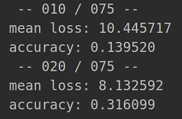
(16)
if (batch_idx+1)%10 == 0:
    log_string(' -- %03d / %03d --' % (batch_idx+1, num_batches))
 log_string('mean loss: %f' % (loss_sum / 10))
 log_string('accuracy: %f' % (total_correct / float(total_seen)))
 total_correct = 0
 total_seen = 0
 loss_sum = 0
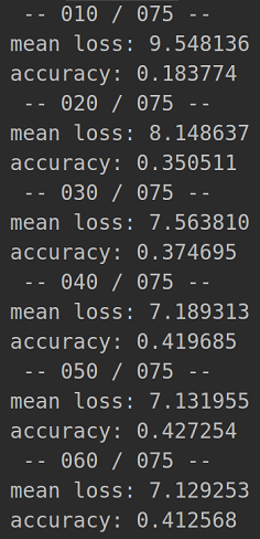
The average loss is calculated once for every 10 batches (1201 / / 16 = 75 batches in total), and the average accuracy is calculated once. 11-20 batches will recalculate the average loss and accuracy of these 11-20 batches.
(17)
It can be seen that the average accuracy rate of the last 10 batches will be higher than that of the first 10 batches, during which the network should constantly self adjust.
(18)
train_one_epoch(sess, ops, train_writer)
Trained an epoch
(19)
for epoch in range(MAX_EPOCH):
            log_string('**** EPOCH %03d ****' % (epoch))
            sys.stdout.flush() #Force flush buffer

            train_one_epoch(sess, ops, train_writer)
            if (epoch+1)%5==0:      #The original code is: if epoch%5==0:
                acc = eval_one_epoch(sess, ops, test_writer)
                acc = eval_whole_scene_one_epoch(sess, ops, test_writer)   #Evaluate the accuracy of the whole scene
            if acc > best_acc:
                best_acc = acc
                save_path = saver.save(sess, os.path.join(LOG_DIR, "best_model_epoch_%03d.ckpt"%(epoch)))
                log_string("Model saved in file: %s" % save_path)
Test every 5 epoch s.
One test was conducted at the 5th, 10th, 15th, 20th, 200 epoch s.
# evaluate on randomly chopped scenes   Evaluation of randomly segmented scenes
def eval_one_epoch(sess, ops, test_writer):
""" ops: dict mapping from string to tf ops """
 global EPOCH_CNT
 is_training = False
 test_idxs = np.arange(0, len(TEST_DATASET)) #312Test scenarios
 num_batches = len(TEST_DATASET)//BATCH_SIZE #Divide the test set into19Batches, each batch contains 16 point sets

 total_correct = 0 #a
 total_seen = 0 #b
 loss_sum = 0 #c
 total_seen_class = [0 for _ in range(NUM_CLASSES)]  #d
 total_correct_class = [0 for _ in range(NUM_CLASSES)]  #e
total_correct_vox = 0 #f
    total_seen_vox = 0 #g
 total_seen_class_vox = [0 for _ in range(NUM_CLASSES)] #h
 total_correct_class_vox = [0 for _ in range(NUM_CLASSES)] #i
a: Number of correctly predicted point clouds
b: Total number of training point clouds
c: Loss. This parameter is used to calculate the average loss of the test set (batchnumber * batchsize * number of pointcloud: 19 * 16 * 8192)
d: Number of point clouds in each category
e: Number of correctly predicted point clouds by category
f: The number of correctly predicted point clouds based on voxels
g: Total number of training point clouds based on voxels
h: Number of point clouds in each category based on voxels
i: The number of correctly predicted point clouds by category -- Based on voxels
correct = np.sum((pred_val == batch_label) & (batch_label>0) & (batch_smpw>0)) # evaluate only on 20 categories but not unknown
Only 20 categories were evaluated, but not unknown.
for l in range(NUM_CLASSES):         #For each category, how many points of each category in a batch are there in total and how many are correctly predicted
            total_seen_class[l] += np.sum((batch_label==l) & (batch_smpw>0))
            total_correct_class[l] += np.sum((pred_val==l) & (batch_label==l) & (batch_smpw>0))
def point_cloud_label_to_surface_voxel_label_fast(point_cloud, label, res=0.0484):
    coordmax = np.max(point_cloud,axis=0)
    coordmin = np.min(point_cloud,axis=0)
    nvox = np.ceil((coordmax-coordmin)/res) #Voxels are magnified 50 times #a.
    vidx = np.ceil((point_cloud-coordmin)/res) #b.
    vidx = vidx[:,0]+vidx[:,1]*nvox[0]+vidx[:,2]*nvox[0]*nvox[1] #c.
    uvidx, vpidx = np.unique(vidx,return_index=True) #d.
    if label.ndim==1:
        uvlabel = label[vpidx]
    else:
        assert(label.ndim==2)
        uvlabel = label[vpidx,:]
    return uvidx, uvlabel, nvox
Parameter 1: point cloud is a point cloud whose weight is not 0 in the point set.
Parameter 2: the actual label and corresponding forecast label of a single test scenario
a. The voxels are magnified 50 times, i.e. length, width and height are magnified 50 times, l × 50=L1, W*50=W1, H × 50=H1
b. After subtracting the minimum coordinates (x-min (x = x1, y-min (y = Y1, z-min (z = z1)) from the test point cloud (x,y,z) (N*3), x1,y1,z1 and Z1 are magnified 50 times respectively, x1*50=x2, y1*50=y2, z1*50=z2
c.x+y * (after the length of the scene bounding box is magnified by 50 times) + z * (after the length of the scene bounding box is magnified by 50 times) * (after the width of the scene bounding box is magnified by 50 times), vidx: n * 3 (for example: 4722 * 3)
Namely: x + y*L1 +z *L1*w1
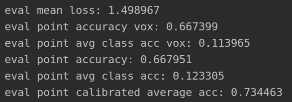
Test result of test set
Average loss:
Voxel accuracy:
Accuracy of average voxels:
Point cloud prediction accuracy:
Average category accuracy:
Weighted average category accuracy:
(20)
The training model is used to evaluate the whole test scenario:
# evaluate on whole scenes to generate numbers provided in the paper
def eval_whole_scene_one_epoch(sess, ops, test_writer):
Loop through each scene:
for batch_idx in range(num_batches): #num_batches=312
        if not is_continue_batch:
            batch_data, batch_label, batch_smpw = TEST_DATASET_WHOLE_SCENE[batch_idx]
For each scene, the point cloud in the voxel with the size of 1.5 × 1.5 × h is extracted circularly (H is the actual height of the scene):
for i in range(nsubvolume_x):
            for j in range(nsubvolume_y):
                curmin = coordmin+[i*1.5,j*1.5,0]
                curmax = coordmin+[(i+1)*1.5,(j+1)*1.5,coordmax[2]-coordmin[2]]
batch_data = batch_data[:BATCH_SIZE,:,:]
            batch_label = batch_label[:BATCH_SIZE,:]
            batch_smpw = batch_smpw[:BATCH_SIZE,:]
The point cloud in the first 16 cubes is taken as a batch of calculation accuracy, and is overlapped with the accuracy of the point cloud in the first 16 cubes of the next scene until 312 scenes are completed. The accumulated accuracy is taken as the prediction accuracy of the whole scene.