Article catalog

• • BP
  • • BP algorithm steps
  • numpy reproduction

BP

1. For the input signal, it should first propagate forward to the hidden layer, and then propagate the output information of the hidden neuron to the output neuron after passing through the action function, and finally output the result.
2. BP network application
   1. Function approximation: train a network with input vector and corresponding output vector to approximate a function;
   2. Pattern recognition: use a specific output vector to associate it with the input vector
   3. Classification: classify the input vectors in a defined and appropriate way;
   4. Data compression: reduce the dimension of output vector to facilitate transmission or storage
3. Requirements for BP action function:
   1. It must be differentiable everywhere, and the binary threshold function {0,1} or symbolic function {- 1, + 1} cannot be used;
   2. BP uses S-type function or hyperbolic tangent function or linear function
   3. S-type function has the function of nonlinear amplification coefficient. It can transform the input signal from negative infinity to positive infinity into 0 to 1 (or - 1 to l)
   4. For the larger input signal, the method coefficient is smaller; For smaller input signals, the amplification factor is larger. The nonlinear input-output relationship can be processed and approximated by using S-type activation function
   5. In the first case, the hidden layer adopts S-type action function, while the output layer adopts linear action function
4. The more hidden layers, the higher the accuracy of the network, but it will affect its generalization ability

BP algorithm steps

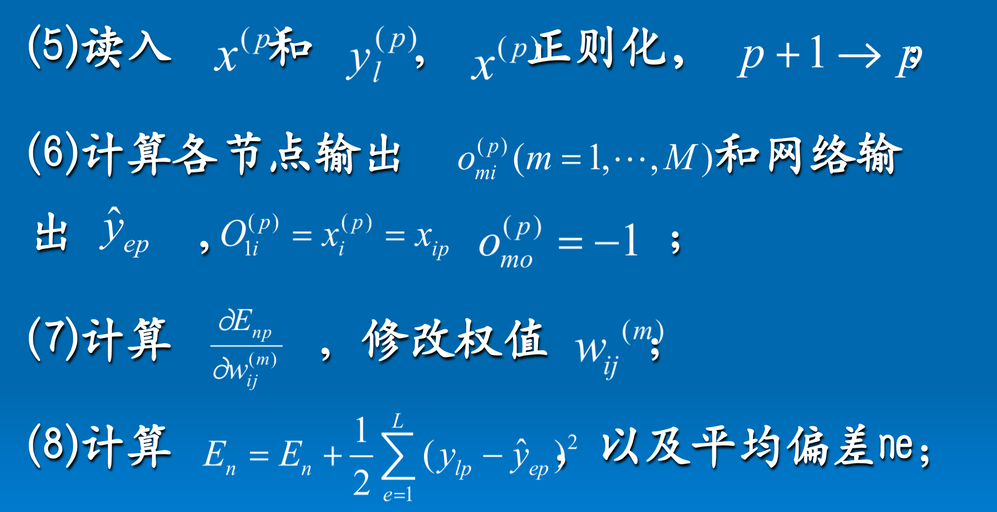
(1) Initialization: \ ETA, \ alpha, pass = 0, Max, me; (2) All weights and neural threshold W are randomly given in the range of [- 0.3,0.3]_ {ij} ^ {(n)} assigns an initial value (3) Judge whether the connection weights of the input terminals of each neuron from layer 2 to layer M of the section meet: Yes turn (4), otherwise reduce to know whether they meet; (4)P = 0,E_{n},pass+1=pass

numpy reproduction

• Title: suppose 7 short segments are used to form a total of 10 digital graphics, so that the 7 segments are represented by a vector [b_1,b_2,b_3,b_4,b_5,b_6,b_7]. For the segments used in the digital graphics, the corresponding component value is 1, and the corresponding component value of the unused segments is 0. Therefore, each digital graphics can be represented by a vector, and its sequence number is 1,2,..., 10, Try to design a neural network, which can distinguish odd numbers from even numbers.

The X matrix is: x = [[1,1,0,0,0,0,0,0], [0,1,1,0,1,1,1], [0,0,1,1,1,1], [1,0,1,1,1,1,1], [1,0,0,1,1,1], [1,1,0,1,1,1], [0,1,1,1,0,0], [1,1,1,1,1,1,1], [1,0,1,1,1,1] The Y tag feature is Y=[1,0,1,0,1,0,1,0,1]

# -*- coding:utf-8 -*-
# /usr/bin/python

import numpy as np
import math

class BP():
    def __init__(self,hidden_n,output_n,learningrate,epoch):
        '''BP parameter'''
        self.hidden_n = hidden_n
        self.output_n = output_n
        self.hideWeight = None
        self.outputWeight = None
        self.learningrate = learningrate
        self.inputN = None
        self.hideOutput = None
        self.output = None
        self.loss= None
        self.epoch = epoch
        self.limitloss = 0.01

    def initWeight(self,n, m,fill=0.0):
        '''Initialization weight'''
        mat = []
        for i in range(m):
            mat.append([fill] * n)
        mat = np.array(mat)
        mat = mat.transpose()
        return mat

    def sigmoid(self,x):
        '''sigmoid Activation function'''
        return 1.0 / (1.0 + np.exp(-x))

    def linear(self,x):
        '''Linear action function'''
        return x

    def sigmoidDerivative(self,x):
        '''Derived sigmoid'''
        return x-x**2

    def initBp(self,inputN):
        '''initialization BP'''
        self.inputN=inputN+1
        self.hideOutput = self.hidden_n+1

        #init weight
        self.hideWeight = self.initWeight(self.inputN,self.hidden_n+1)
        self.outputWeight = self.initWeight(self.hidden_n+1,self.output_n)

    def forwardPropagation(self,X):
        '''Forward propagation'''
        self.hideOutput = self.sigmoid(np.dot(X,self.hideWeight))
        # self.hideOutput = np.c_[self.hideOutput, np.ones(self.hideOutput.shape[0])]# Add a column for bias
        self.output = self.sigmoid(np.dot(self.hideOutput, self.outputWeight))

    def lossFun(self,Y):
        '''loss function '''
        self.loss = 0.5*np.sum((Y - self.output) * (Y - self.output))
        return self.loss

    def backPropagation(self,X,Y):
        self.outputWeight = self.outputWeight.transpose()
        outputWeightbiassum= 0
        for i in range(self.output_n):
            outputWeightbias = self.learningrate * (self.output[i] - Y[i]) * self.sigmoidDerivative(self.output[i]) * self.hideOutput
            self.outputWeight[i,:] +=  outputWeightbias
            outputWeightbiassum -= outputWeightbias
        self.outputWeight = self.outputWeight.transpose()

        self.hideWeight = self.hideWeight.transpose()
        for i in range(self.hidden_n+1):
            hideWeightbias = self.learningrate*outputWeightbias[i]*self.sigmoidDerivative(self.hideOutput[i])*X
            self.hideWeight[i, :] -= hideWeightbias
        self.hideWeight = self.hideWeight.transpose()

    def train(self,X,Y):
        '''train'''
        inputN = X.shape[1]
        samplesN= X.shape[0]
        X = np.c_[X,np.ones(samplesN)] # Add a column for bias
        self.initBp(inputN)
        for i in range(self.epoch):
            for one in range(samplesN):
                x,y = X[one,:],Y[one,:]
                self.forwardPropagation(x)
                loss = self.lossFun(y)
                if loss<= self.limitloss:
                    break
                else:
                    self.backPropagation(x,y)
                i +=1

    def predict(self,X):
        '''forecast'''
        samplesN = X.shape[0]
        X = np.c_[X, np.ones(samplesN)]  # Add a column for bias
        for one in range(samplesN):
            x= X[one, :]
            self.forwardPropagation(x)
            print(self.output)

X=[[1,1,0,0,0,0,0],[0,1,1,0,1,1,1],[0,0,1,1,1,1,1],[1,0,1,1,0,1,0],[1,0,0,1,1,1,1],[1,1,0,1,1,1,1],[0,0,1,1,1,0,0],[1,1,1,1,1,1,1],[1,0,1,1,1,1,1]]
Y=[[1],[0],[1],[0],[1],[0],[1],[0],[1]]

xtest = [[1,1,0,0,0,0,0],[0,1,1,0,1,1,1]]
print(X,"\n",Y)
XTrain = np.array(X)
YTrain = np.array(Y)
xtest = np.array(xtest)
print(XTrain.shape[1])
print(XTrain)

hidden_n,output_n,learningrate,epoch = 3,1,0.5,1000
newbp = BP(hidden_n,output_n,learningrate,epoch)
newbp.train(XTrain,YTrain)
newbp.predict(xtest)