This includes three parts:
- Simple self encoder
- Convolutional self encoder
- Denoising self encoder
catalogue
Decoder: transpose convolution
(additional) decoder: upper sampling layer + convolution layer
1 simple self encoder
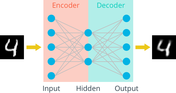
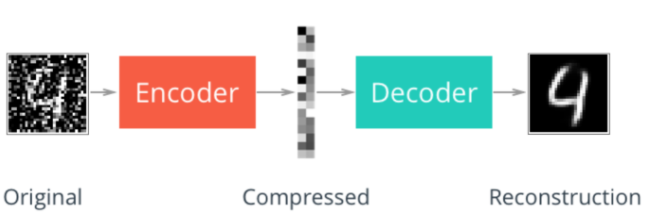
First, we will build a simple automatic encoder to compress MNIST data set. Using the automatic encoder, we transmit the input data through the encoder, which compresses the input data. The representation then reconstructs the input data through a decoder. Generally, the encoder and decoder will be used together with the neural network, and then the sample data will be trained.
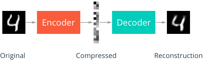
Compression representation
Compressed representation is ideal for saving and sharing any type of data in a more efficient way than storing raw data. In practice, compressed representation usually saves key information about the input image, and we can use it to denoise the image or other types of reconstruction and transformation!
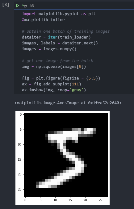
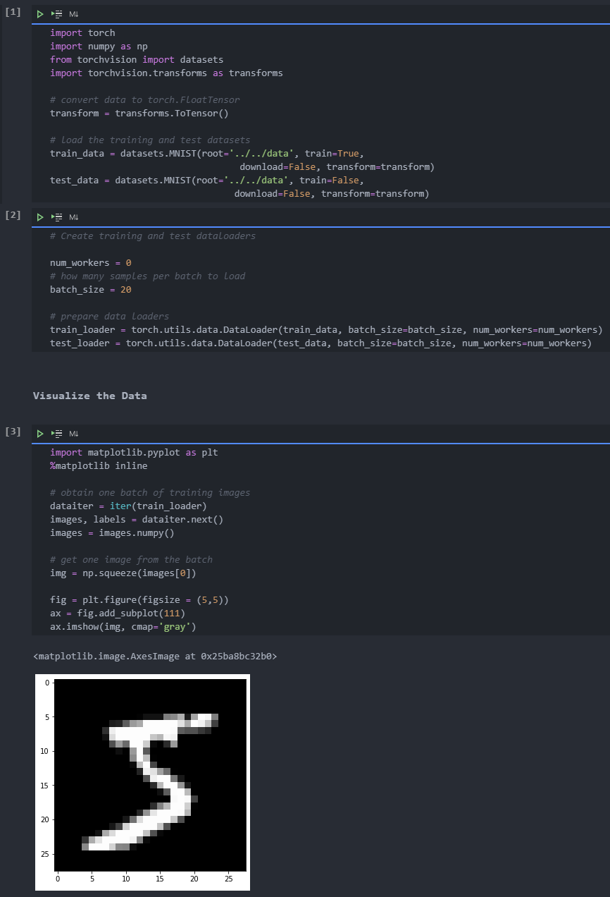
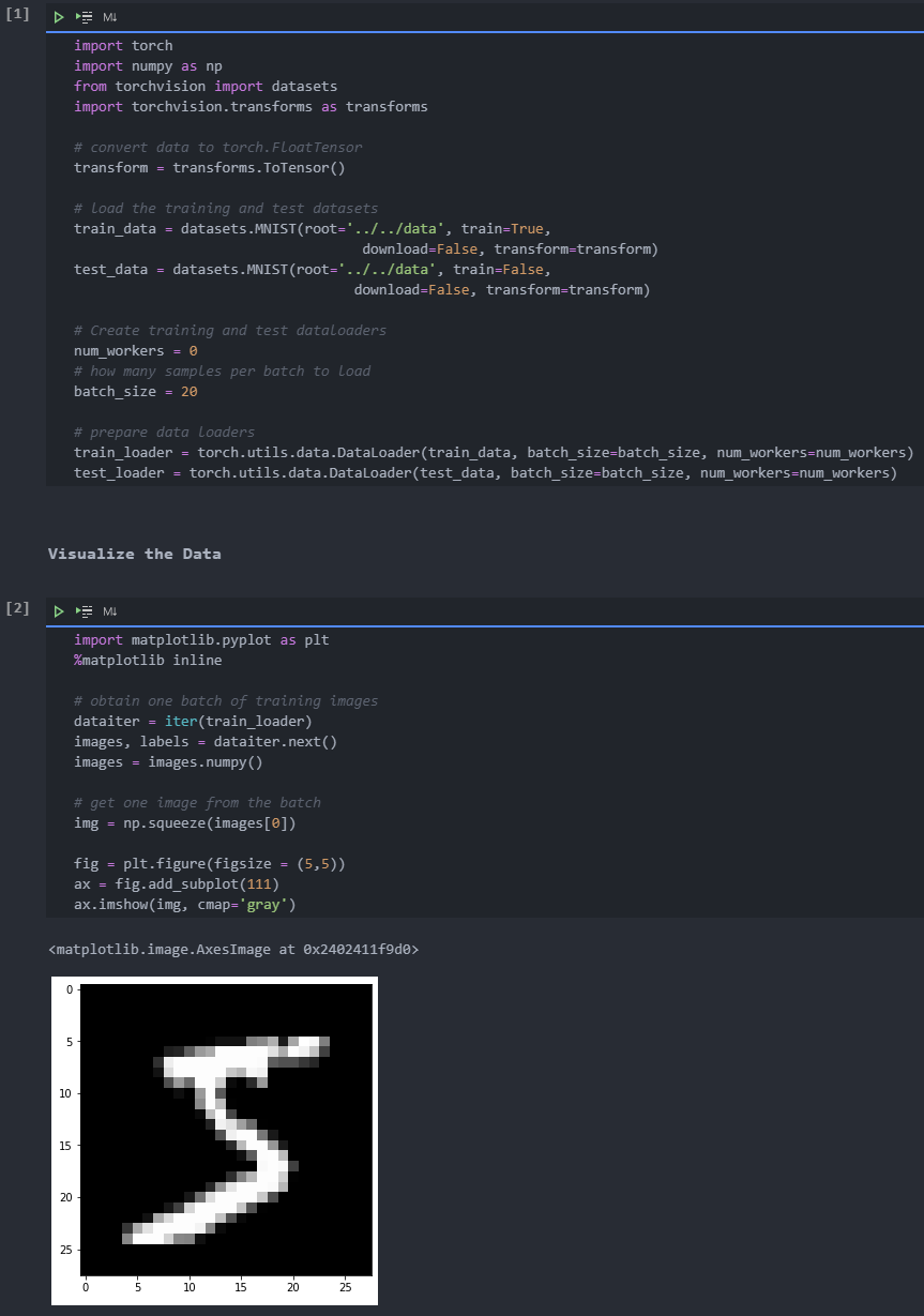
In this notebook, we will build a simple network architecture for encoder and decoder. Let's start importing the library and get the dataset.
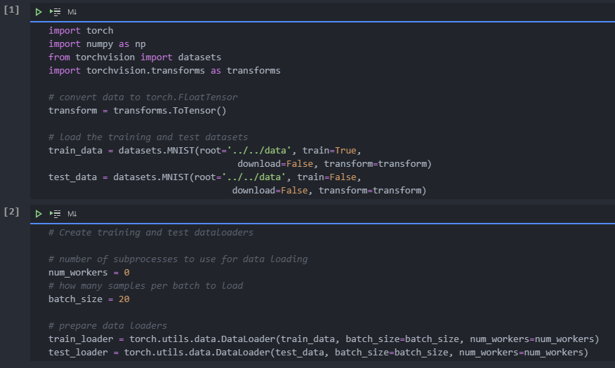
Visual data
Linear self encoder
We will use these images to train an automatic encoder and flatten them into a vector of 784 length. The images from this dataset have been normalized with values between 0 and 1. Let's start by building a simple automatic encoder. The encoder and decoder shall consist of a linear layer. The unit connecting the encoder and decoder will be a compressed representation.
Since the image is standardized between 0 and 1, we need to use sigmoid activation on the output layer to obtain the value matching the input value range.
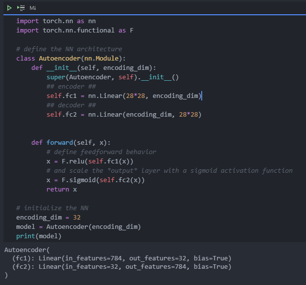
To do: build a chart for the automatic encoder in the following cells.
- The input image will be flattened to a vector of 784 length. The target is the same as the input. The encoder and decoder will consist of two linear layers. The depth dimension should be changed as follows: 784 inputs > encoding_ dim > 784 outputs. All layers will apply ReLu activation, except for the final output layer, which has a sigmoid activation.
compressed representation should be an encoding dimension_ Vector with dim = 32.
train
Here, I will write some code to train the network. I am not very interested in verification here, so I will monitor the training loss and test loss later.
In this example, we don't care about labels, we only care about images. We can learn from train_ Get the image in the loader. Because we are comparing the pixel values in the input and output images, it is best to use the loss function for the regression task. Regression is about comparing quantities, not probability values. In this case, I will use mselos. The output image and the input image are compared as follows:
In addition, this is a very simple PyTorch training. We flatten the image, input it into the automatic encoder, and record the loss in the training process.
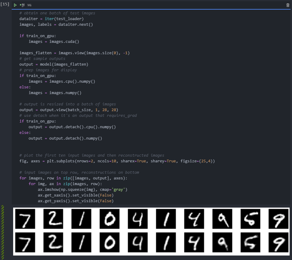
Inspection results
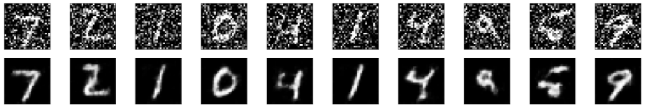
Below I draw some test images and their reconstruction. In most cases, these look good, except for some vague parts.
Next section
We're dealing with images here, so we can (usually) use convolution layers for better performance. So next, we will use convolution layer to build a better automatic encoder.
2 convolutional self encoder
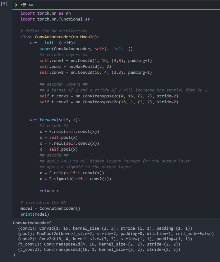
Continuing with the MNIST dataset, let's use the convolution layer to improve the performance of the automatic encoder. We will build a convolutional automatic encoder to compress MNIST data set.
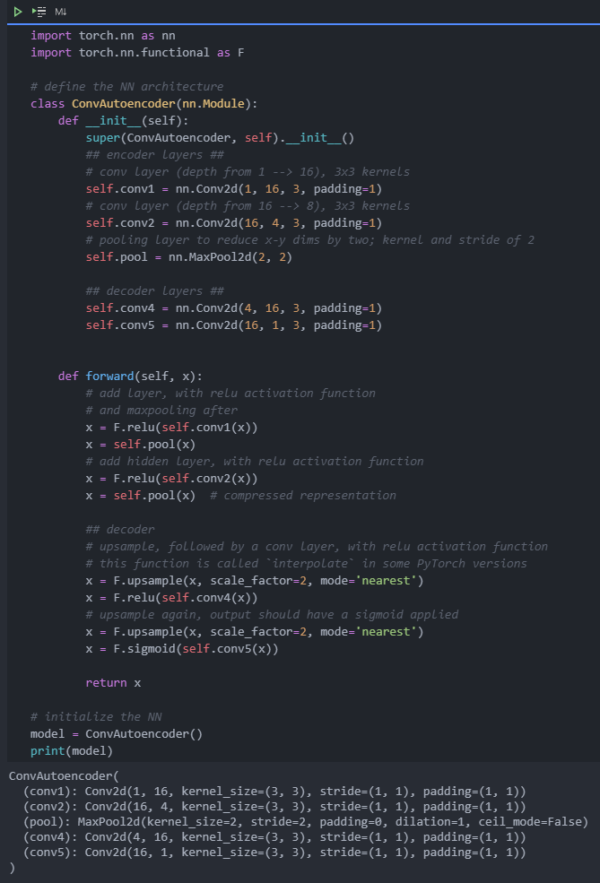
The encoder part will consist of convolution and pooling layers, and the decoder will consist of transposed convolution layers that learn the "up sampling" compression representation.

Encoder
The encoder part of the network will be a typical convolution pyramid. There is a maximum pool layer behind each convolution layer to reduce the dimension of the layer.
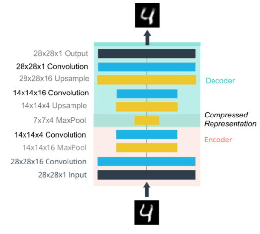
Decoder
But this decoder may be new to you. The decoder needs to convert from a narrow representation to a wide, reconstructed image. For example, the representation can be a max pool layer of 7x7x4. This is the output of the encoder and the input of the decoder. We want to get a 28x28x1 image from the decoder, so we need to return from the compressed representation. The schematic diagram of the network is shown below.
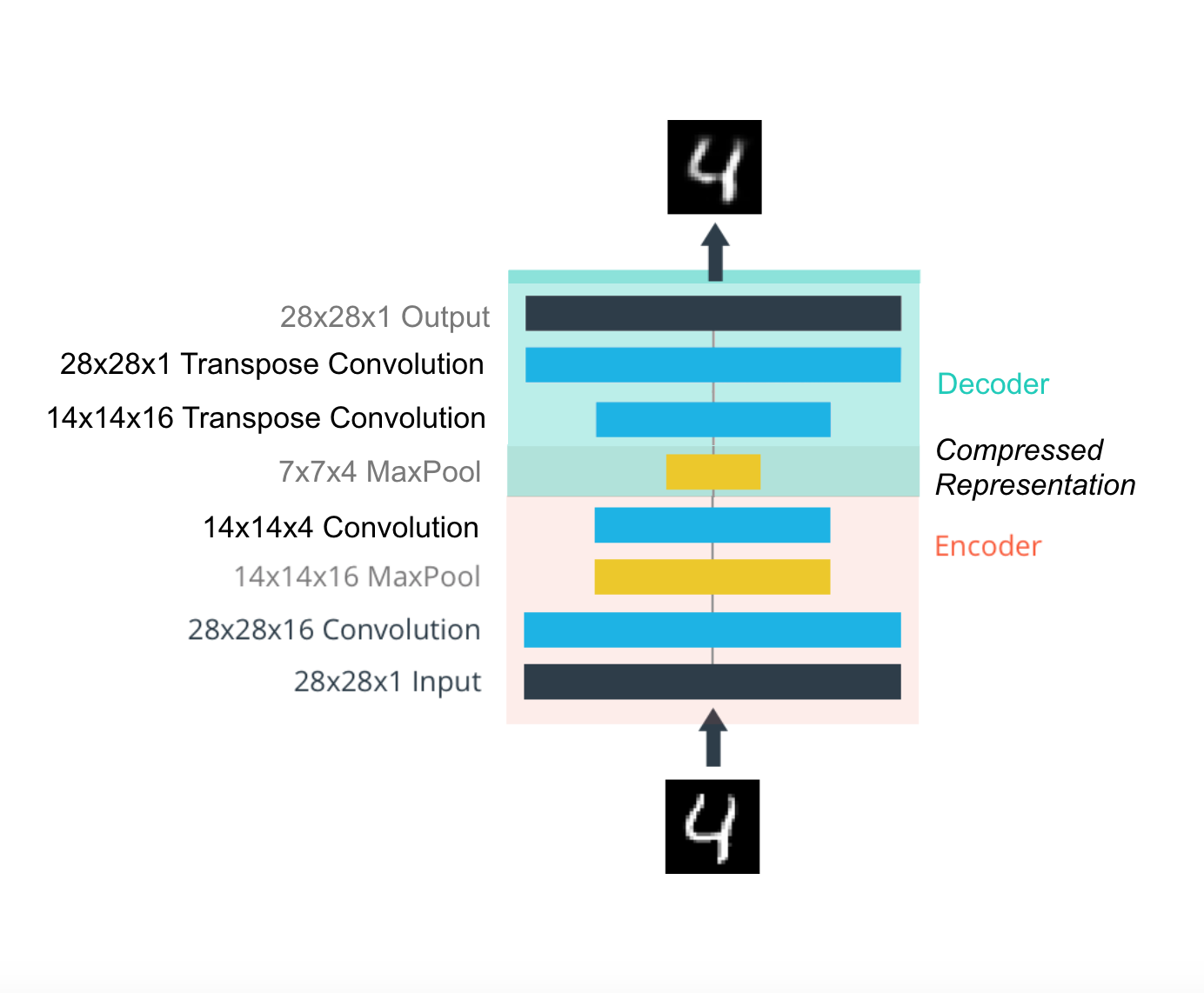
Here, the size of our final encoder layer is 7x7x4 = 196. The size of the original image is 28x28 = 784, so the encoded vector is 25% of the size of the original image. These are only the recommended dimensions for each floor. You can change the depth and size at will. In fact, we encourage you to add additional layers to make this performance smaller! Remember, our goal here is to find a small representation of the input data.
Decoder: transpose convolution
The decoder uses a transposed convolution layer to increase the width and height of the input layer. Their working principle is almost the same as that of convolution layer, but in the opposite way. The stride of the input layer causes the stride of the convolution layer to be transposed. For example, if you have a 3x3 kernel, a 3x3 patch in the input layer will be simplified to a unit in a volume layer. In contrast, a unit in the input layer will be expanded to transpose 3x3 patch in the convolution layer. PyTorch gives us a simple way to create layers NN ConvTranspose2d.
It is worth noting that transposing the convolution layer may lead to artifacts in the final image, such as checkerboard patterns. This is due to the overlap in the kernel, which can be avoided by setting the stride equal to the kernel size. In this Distill article by Augustus Odena et al., the author points out that these checkerboard effects can be avoided by using nearest neighbor or bilinear interpolation (up sampling) and then using convolution layer to adjust the layer size.
- We will show this method in another notebook so that you can experiment with it and see the difference.
To do: establish the network shown above.
- The encoder is constructed with a series of convolution and pooling layers. When building the decoder, remember that the transpose convolution layer can use stripe and kernel_size=2 to sample up the input.
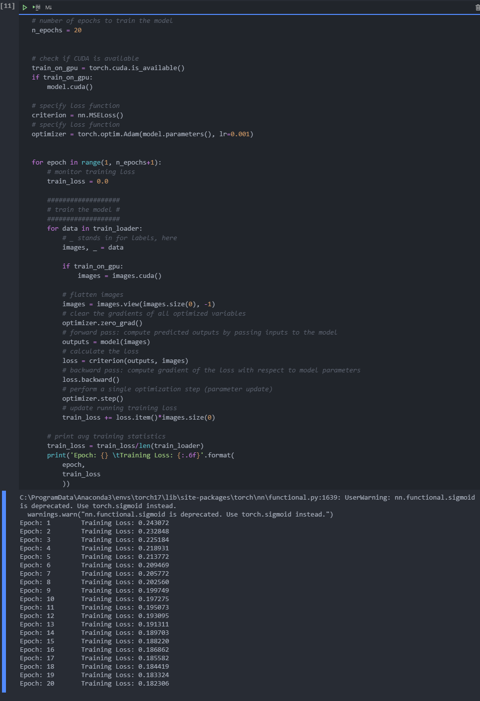
train
# specify loss function
criterion = nn.MSELoss()

# specify loss function
optimizer = torch.optim.Adam(model.parameters(), lr=0.001)


# number of epochs to train the model
n_epochs = 30

for epoch in range(1, n_epochs+1):
    # monitor training loss
    train_loss = 0.0

    ###################
    # train the model #
    ###################
    for data in train_loader:
        # _ stands in for labels, here
        # no need to flatten images
        images, _ = data
        # clear the gradients of all optimized variables
        optimizer.zero_grad()
        # forward pass: compute predicted outputs by passing inputs to the model
        outputs = model(images)
        # calculate the loss
        loss = criterion(outputs, images)
        # backward pass: compute gradient of the loss with respect to model parameters
        loss.backward()
        # perform a single optimization step (parameter update)
        optimizer.step()
        # update running training loss
        train_loss += loss.item()*images.size(0)

    # print avg training statistics
    train_loss = train_loss/len(train_loader)
    print('Epoch: {} \tTraining Loss: {:.6f}'.format(
        epoch,
        train_loss
        ))
result:
Epoch: 1 	Training Loss: 0.536067
Epoch: 2 	Training Loss: 0.296300
Epoch: 3 	Training Loss: 0.271992
Epoch: 4 	Training Loss: 0.257491
Epoch: 5 	Training Loss: 0.248846
Epoch: 6 	Training Loss: 0.242581
Epoch: 7 	Training Loss: 0.238418
Epoch: 8 	Training Loss: 0.235051
Epoch: 9 	Training Loss: 0.232203
Epoch: 10 	Training Loss: 0.230150
Epoch: 11 	Training Loss: 0.228493
Epoch: 12 	Training Loss: 0.226843
Epoch: 13 	Training Loss: 0.225579
Epoch: 14 	Training Loss: 0.224565
Epoch: 15 	Training Loss: 0.223704
Epoch: 16 	Training Loss: 0.222844
Epoch: 17 	Training Loss: 0.221671
Epoch: 18 	Training Loss: 0.220569
Epoch: 19 	Training Loss: 0.219486
Epoch: 20 	Training Loss: 0.218675
Epoch: 21 	Training Loss: 0.218025
Epoch: 22 	Training Loss: 0.217432
Epoch: 23 	Training Loss: 0.216864
Epoch: 24 	Training Loss: 0.216343
Epoch: 25 	Training Loss: 0.215857
Epoch: 26 	Training Loss: 0.215377
Epoch: 27 	Training Loss: 0.214942
Epoch: 28 	Training Loss: 0.214570
Epoch: 29 	Training Loss: 0.214245
Epoch: 30 	Training Loss: 0.213977
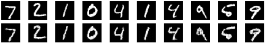
Inspection results
Below I draw some test images and their reconstruction. These seemingly rough edges may be due to the chessboard effect mentioned above, which often occurs in the transpose layer.
Training results:
Epoch: 1 	Training Loss: 0.323222
Epoch: 2 	Training Loss: 0.167930
Epoch: 3 	Training Loss: 0.150233
Epoch: 4 	Training Loss: 0.141811
Epoch: 5 	Training Loss: 0.136143
Epoch: 6 	Training Loss: 0.131509
Epoch: 7 	Training Loss: 0.126820
Epoch: 8 	Training Loss: 0.122914
Epoch: 9 	Training Loss: 0.119928
Epoch: 10 	Training Loss: 0.117524
Epoch: 11 	Training Loss: 0.115594
Epoch: 12 	Training Loss: 0.114085
Epoch: 13 	Training Loss: 0.112878
Epoch: 14 	Training Loss: 0.111946
Epoch: 15 	Training Loss: 0.111153
Epoch: 16 	Training Loss: 0.110411
Epoch: 17 	Training Loss: 0.109753
Epoch: 18 	Training Loss: 0.109152
Epoch: 19 	Training Loss: 0.108625
Epoch: 20 	Training Loss: 0.108119
Epoch: 21 	Training Loss: 0.107637
Epoch: 22 	Training Loss: 0.107156
Epoch: 23 	Training Loss: 0.106703
Epoch: 24 	Training Loss: 0.106221
Epoch: 25 	Training Loss: 0.105719
Epoch: 26 	Training Loss: 0.105286
Epoch: 27 	Training Loss: 0.104917
Epoch: 28 	Training Loss: 0.104582
Epoch: 29 	Training Loss: 0.104284
Epoch: 30 	Training Loss: 0.104016
Codec effect:
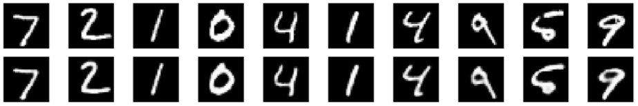
(additional) decoder: upper sampling layer + convolution layer
The decoder uses the combination of the nearest neighbor upper sampling layer and the normal convolution layer to increase the width and thickness of the input layer.
To do: establish a network as shown below.
- The encoder is constructed with a series of convolution and pooling layers. When constructing the decoder, the combination of up sampling and normal convolution layer is used.
3 denoising self encoder
Continue to use MNIST data set. Let's add noise to the data and see if we can define and train an automatic encoder for denoising.
Let's start importing the library and get the dataset.
Denoising
As I mentioned earlier, an automatic encoder like the one you are currently building is not very useful in practice. However, as long as the network is trained on the noisy image, it can be successfully used for image denoising. We can create a noisy image by adding Gaussian noise to the training image, and then crop it to between 0 and 1.
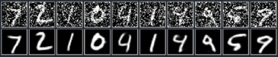
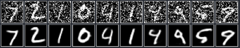
- We will use noise image as input and original and clean image as label.
Here are some examples of noise images and related denoising images I generated.
Because this is a more difficult problem for the network, we want to use a deeper convolution layer here; Layers with more functional maps. You can also consider adding additional layers. I suggest setting the depth of the convolution layer in the encoder to 32 and pushing the same depth back into the decoder.
TODO: build the network of denoising self encoder. Add deeper and / or more layers than the above model.
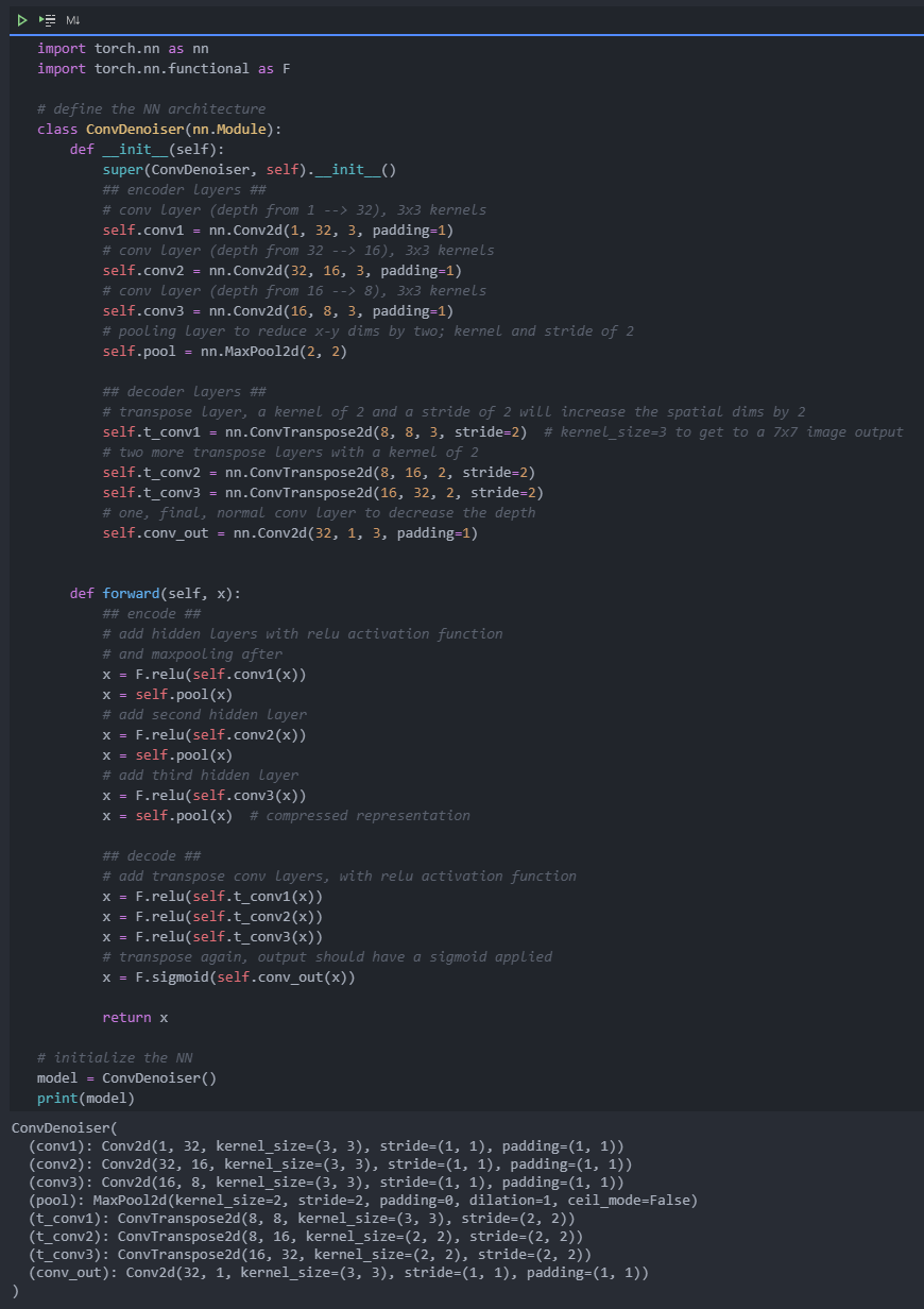
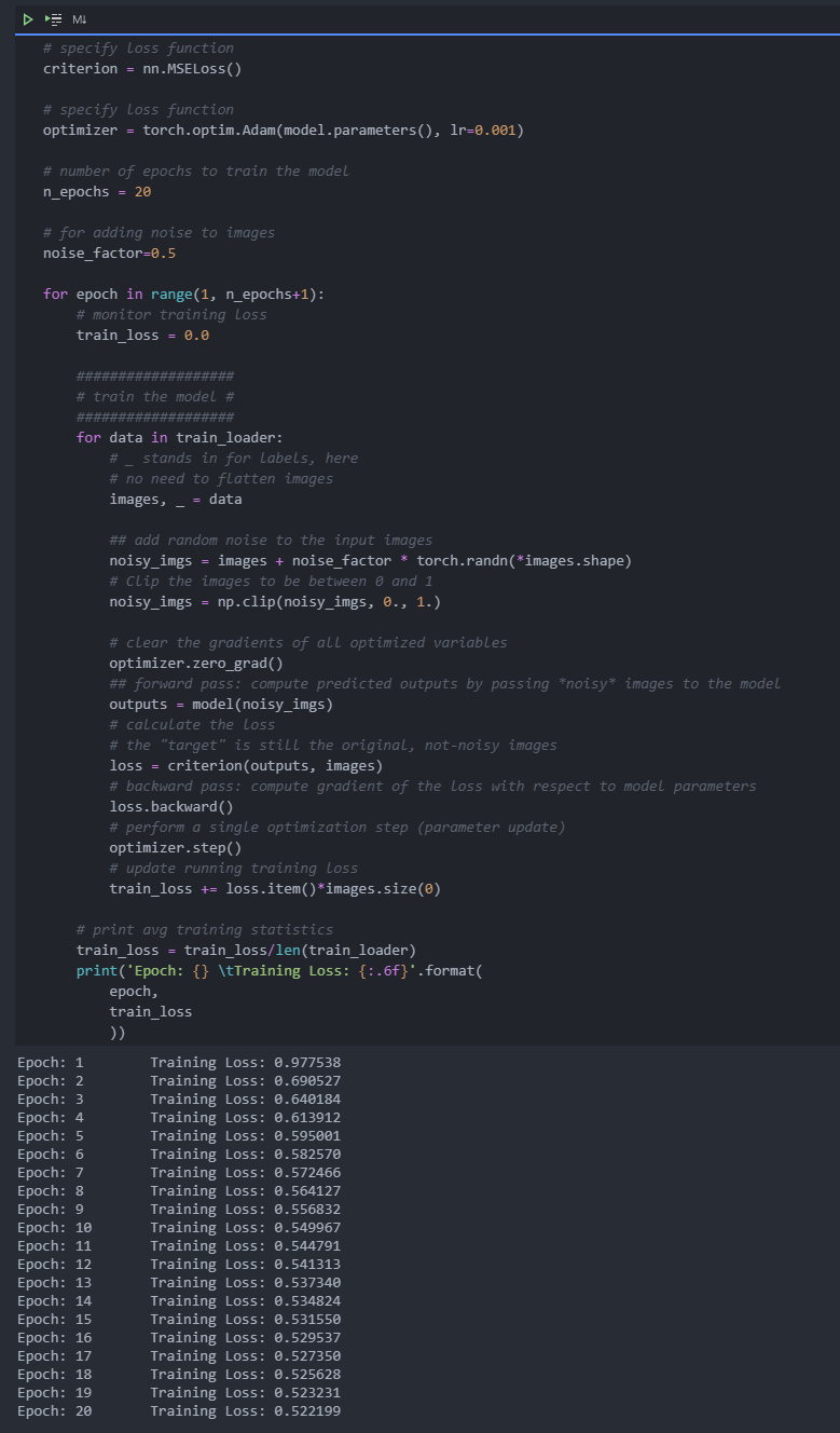
train
We only care about what we can do from train_ The training image obtained in the loader.
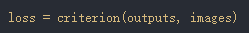
In this case, we actually add some noise to these images and add the noise y_ The model provided to us by IMGs. The model will produce a reconstructed image based on noise input. However, we want it to produce a normal noise free image, so when we calculate the loss, we will still compare the reconstructed output with the original image!
Because we are comparing the pixel values in the input and output images, it is best to use the loss function for the regression task. In this case, I will use mselos. The output image and the input image are compared as follows:
Check the denoising effect