Catalog

 

Direct Singular Value Decomposition of Matrix

Compressed image decomposition using SVD

Solution of Overdetermined Equation by SVD Decomposition

Direct Singular Value Decomposition of Matrix

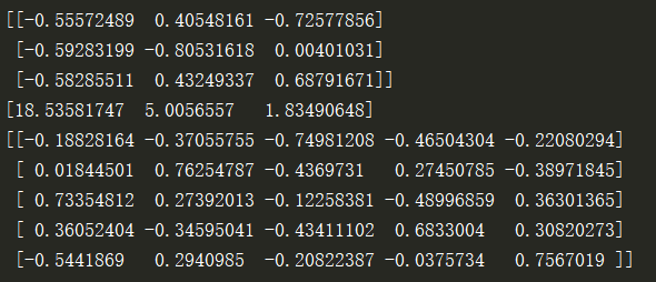
Known matrixSingular value decomposition is performed.

import numpy as np
#Create A
A = np.array([[1,5,7,6,1],[2,1,10,4,4],[3,6,7,5,2]])

#Direct singular value decomposition using np.linalg.svd() function
#The function has three return values: left singular matrix, all singular values and right singular matrix.
U,Sigma,VT = np.linalg.svd(A)

#Exhibition
print(U)
print(Sigma)
print(VT)

Operation results:

Compressed image decomposition using SVD

Original image:

Code:

import matplotlib.pyplot as plt
import matplotlib.image as mpimg
import numpy as np

img_eg = mpimg.imread("car.jpg")
print(img_eg.shape) #Operation results: (400,640,3)


#Converting image data into two-dimensional matrix and singular value decomposition
img_temp = img_eg.reshape(400, 640 * 3)
U,Sigma,VT = np.linalg.svd(img_temp)

# Take the first 10 singular values
sval_nums = 10
img_restruct1 = (U[:,0:sval_nums]).dot(np.diag(Sigma[0:sval_nums])).dot(VT[0:sval_nums,:])
img_restruct1 = img_restruct1.reshape(400,640,3)
img_restruct1.tolist()

# Take the first 50 singular values
sval_nums = 50
img_restruct2 = (U[:,0:sval_nums]).dot(np.diag(Sigma[0:sval_nums])).dot(VT[0:sval_nums,:])
img_restruct2 = img_restruct2.reshape(400,640,3)

# Take the first 100 singular values
sval_nums = 100
img_restruct3 = (U[:,0:sval_nums]).dot(np.diag(Sigma[0:sval_nums])).dot(VT[0:sval_nums,:])
img_restruct3 = img_restruct3.reshape(400,640,3)

#Exhibition
fig, ax = plt.subplots(nrows=1, ncols=3)
ax[0].imshow(img_restruct1.astype(np.uint8))
ax[0].set(title = "10")
ax[1].imshow(img_restruct2.astype(np.uint8))
ax[1].set(title = "50")
ax[2].imshow(img_restruct3.astype(np.uint8))
ax[2].set(title = "100")
plt.show()

Operation results:

It can be seen that the first 50 or 100 eigenvalues can be used to reconstruct the image, which saves a lot of space compared with the original image (400 eigenvalues).

Solution of Overdetermined Equation by SVD Decomposition

So for homogeneous linear equationsIfFull rank andThen the equations are overdetermined (the number of effective equations is greater than the number of unknown parameters). At this time, the equations have no exact solution, so the least square solution needs to be solved. stayUnder the constraints of the matrix, the least square solution is a matrix.The minimum eigenvalue corresponds to the eigenvector.

In this way, we can solve a very simple overdetermined system of equations.

First of all, we simplify this system of equations toFormat:

Here is the code:

import numpy as np
#Input coefficient matrix A
A = np.array([[2,4,-11],[3,-5,-3],[1,2,-6],[2,1,-7]])


#svd decomposition of A
U,Sigma,VT = np.linalg.svd(A)
#print(U)
#print(Sigma)
#print(VT)

#The column vector of V is the eigenvector of ATA.
#The row vector of the last line of VT is the eigenvector corresponding to the minimum eigenvalue.
#Because x[3,0]=1, the results need to be processed
k=1/ VT[2,2]
x_1=VT[2,0]*k
x_2=VT[2,1]*k
print(x_1,x_2)

#error
X=np.array([[x_1],[x_2],[1]])
R=np.dot(np.transpose(np.dot(A,X)),(np.dot(A,X)))
print (R)

Operation results:

The least squares solution isThe sum of squares of errors.