preface

Decision tree is a common algorithm in machine learning. Relevant mathematical theories I also wrote in the column of mathematical modeling Mathematical modeling learning notes (XXV) decision tree
Yes, this blog post does not pay attention to the relevant mathematical principles, but mainly focuses on the effect of using sklearn to realize the classification tree.
For reference courses, see [2020 complete collection of machine learning] sklearn complete version of vegetables

Introduction to decision tree

Decision Tree is a nonparametric supervised learning method. It can summarize decision rules from a series of characteristic and labeled data, and present these rules with the structure of tree view to solve the problems of classification and regression.

Decision tree in sklearn

• Module sklearn.tree

Tree type	Library representation
Classification tree	tree.DecisionTreeClassifier
Regression tree	tree.DecisionTreeRegressor
The generated decision tree is exported to DOT format for drawing	tree.export_graphviz
High random version classification tree	tree.ExtraTreeClassifier
High random version of regression tree	tree.ExtraTreeRegressor

Basic modeling process of sklearn

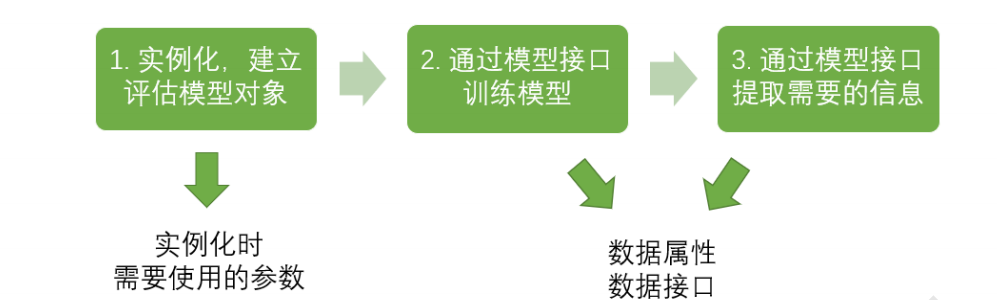
Corresponding python code

from sklearn import tree #Import required modules

clf = tree.DecisionTreeClassifier()     #instantiation 
clf = clf.fit(X_train,y_train) #Training model with training set data
result = clf.score(X_test,y_test) #Import the test set and call the required information from the interface.

Classification tree DecisionTreeClassifier

Important parameters

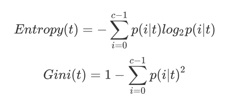
criterion determines the calculation method of impurity

In order to transform the table into a tree, the decision tree needs to find the best node and the best branching method. For the classification tree, the index to measure this "best" is called "impure". Generally speaking, the lower the purity, the better the fitting of the decision tree to the training set.
Popular understanding: in order to separate a group of complex samples mixed together, it is measured by impure. Before the score, that is, the root node, the impure is the highest, and then the lower the impure is, to the leaf node, it is completely separated. The impure is the lowest, and the result is the most "pure"!

The Criterion parameter is used to determine the calculation method of impurity. sklearn offers two options:
1) Enter "entropy" to use information entropy
2) Enter "gini" to use gini impulse

Do not fill in. The default is gini.
sklearn actually calculates the information gain based on information entropy, that is, the difference between the information entropy of the parent node and the information entropy of the child node.

Selection rules:
Gini coefficient is usually used
Gini coefficient is used when the data dimension is large and the noise is large
When the dimension is low and the data is clear, there is no difference between information entropy and Gini coefficient
When the fitting degree of decision tree is not enough, information entropy is used
Try both. If not, change the other one

To create a classification tree

1. Import the required algorithm libraries and modules

from sklearn import tree
from sklearn.datasets import load_wine
from sklearn.model_selection import train_test_split
import pandas as pd
import graphviz

2. View data
The wine dataset provided by sklearn is used here.

wine = load_wine()
print(wine.data.shape)

print(pd.concat([pd.DataFrame(wine.data), pd.DataFrame(wine.target)], axis=1))
print(wine.feature_names)
print(wine.target_names)

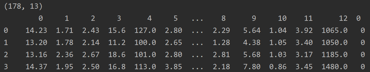
A total of 178 data, 3 classification problems.

3. Divide training set and test set

Xtrain, Xtest, Ytrain, Ytest = train_test_split(wine.data,wine.target,test_size=0.3)
print(Xtrain.shape)
print(Xtest.shape)

test_size=0.3 means that the test set accounts for 30% of the sample number

After division, the training set is 124 data and the test set is 54 data.

4. Model establishment

clf = tree.DecisionTreeClassifier(criterion="entropy")
clf = clf.fit(Xtrain, Ytrain)
score = clf.score(Xtest, Ytest) # Returns the accuracy of the forecast
print(score)

Here, entropy is selected as the calculation method.
score stands for accuracy
Because the establishment of decision tree contains random variables, the results are different every time.
Here I run several times, and the accuracy of the approximate results is more than 90%.

5. Decision tree visualization

feature_name = ['alcohol','malic acid','ash','Alkalinity of ash','magnesium','Total phenol','flavonoid','Non flavane phenols','anthocyanin','Color intensity','tone','od280/od315 Diluted wine','proline']

dot_data = tree.export_graphviz(clf
                               ,feature_names= feature_name
                               ,class_names=["Type I","Type II","Type III"]
                               ,filled=True  #Control color fill
                               ,rounded=True  #Controls whether the picture is rounded
                               )
graph = graphviz.Source(dot_data.replace('helvetica','"Microsoft YaHei"'), encoding='utf-8')
graph.view()

An error will be reported when running directly here. The problem is that although the graphviz library is installed, the graphviz plug-in still needs to be installed to display pictures.
Plug in download address https://graphviz.gitlab.io/download/
windows select:

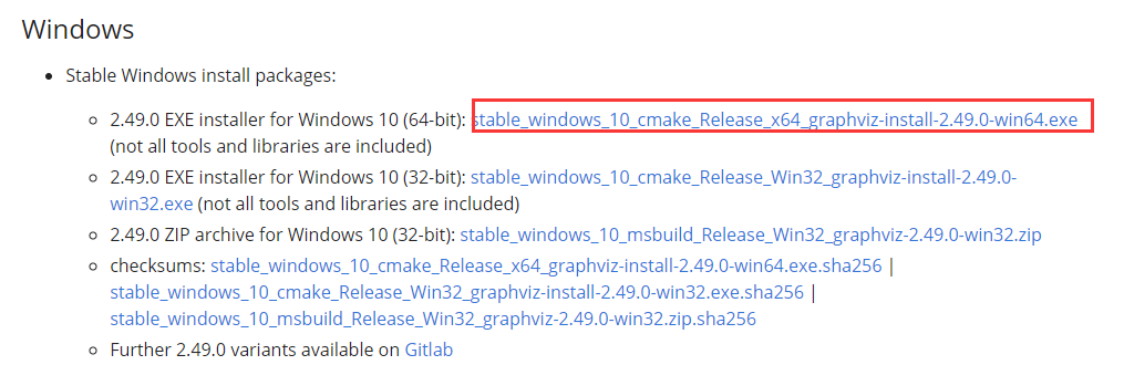
During installation, check add graphviz to environment variable

replace('helvetica ',' Microsoft YaHei '), encoding='utf-8' aims to prevent Chinese garbled code and use UTF-8 for re encoding.

After running, a pdf image will be opened directly.

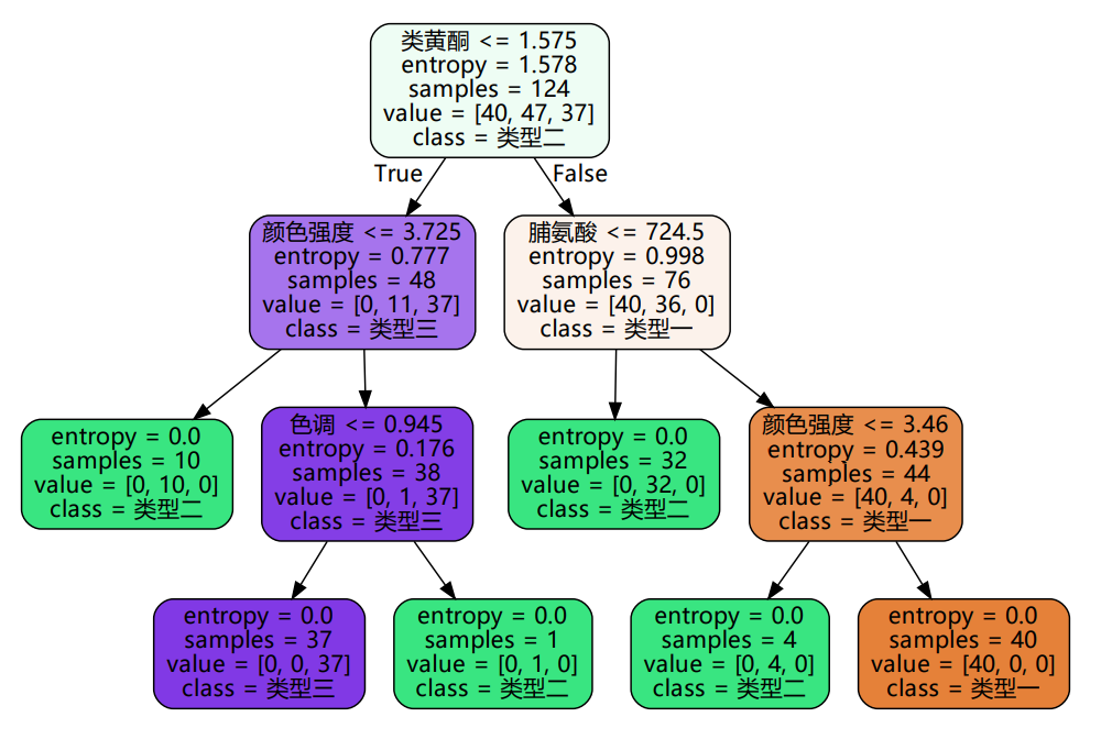
This is the classification decision tree. The first row on each branch node represents the basis of branches.
The color represents the impurity, the darker the color represents the smaller the impurity, and the leaf node impurity is 0.

6. Feature importance display
The decision tree branch in the figure above is based on the feature importance (information gain). The importance of each feature can be printed through the following program.

print([*zip(feature_name,clf.feature_importances_)])

Results obtained:

[('alcohol', 0.0), ('malic acid', 0.0), ('ash', 0.0), ('Alkalinity of ash', 0.03448006546085971), ('magnesium', 0.0), ('Total phenol', 0.0), ('flavonoid', 0.4207777417026953), ('Non flavane phenols', 0.0), ('anthocyanin', 0.0), ('Color intensity', 0.1444829682905809), ('tone', 0.03408453152321241), ('od280/od315 Diluted wine', 0.0), ('proline', 0.3661746930226517)]

The importance of some features is 0, indicating that these indicators are not used in the decision tree.

Random parameter_ state & splitter

In the above example, the results will be different each time. The reason is that when using the decision tree provided by sklearn, it will "plant" several different decision trees by default, and return the one with the best effect.

random_state is used to set the parameters of the random mode in the branch. The default is None. If you enter any integer, the same tree will grow all the time to stabilize the model.

splitter is also used to control random options in the decision tree. There are two input values:

• Enter "best". Although the decision tree is randomly branched, it will preferentially select more important features for branching (importance can be determined by attribute feature)_ importances_ (view)
• Enter "random", the decision tree will be more random when branching, the tree will be deeper and larger because it contains more unnecessary information, and the fitting of the training set will be reduced because of these unnecessary information. This is also a way to prevent over fitting.

clf = tree.DecisionTreeClassifier(criterion="entropy"
                                 ,random_state=30
                                 ,splitter="random"
                                 )

Setting random parameters can make the decision tree stable or more random, and the effect is uncertain. Everything is dominated by the final score.

Pruning strategy max_depth

max_depth is used to limit the maximum depth of the tree, and all branches exceeding the set depth are cut off
If the policy tree grows one more layer, the demand for sample size will double.
In actual use, it is recommended to try from = 3 to see the fitting effect, and then decide whether to increase the set depth.

Pruning strategy min_ samples_ leaf & min_ samples_ split

min_samples_leaf defines that each child node of a node after branching must contain at least min_ samples_ Leave training samples, otherwise score
Branches will not occur. Generally speaking, it is recommended to start from = 5.

min_samples_split limit, a node must contain at least min_samples_split training samples, this node is allowed to be branched, otherwise
Branching doesn't happen.

clf = tree.DecisionTreeClassifier(criterion="entropy"
                                 ,random_state=30
                                 ,splitter="random"
                                 ,max_depth=3
                                 ,min_samples_leaf=10
                                 ,min_samples_split=10
                                 )

Pruning strategy Max_ features & min_ impurity_ decrease

max_features limits the number of features considered when branching, and features exceeding the limit will be discarded.

min_impurity_decrease limits the size of information gain. Branches with information gain less than the set value will not occur.

Confirm the optimal pruning parameters

Through programming cycle, other quantities are controlled to remain unchanged, a quantity cycle is changed, and the optimal value of this quantity can be displayed by drawing and displaying.

Below is max_depth as an example:

import matplotlib.pyplot as plt

test = []
for i in range(10):
    clf = tree.DecisionTreeClassifier(max_depth=i+1
                                     ,criterion="entropy"
                                     ,random_state=30
                                     ,splitter="random"
                                     )
    clf = clf.fit(Xtrain, Ytrain)
    score = clf.score(Xtest, Ytest)
    test.append(score)
plt.plot(range(1,11),test,color="red",label="max_depth")
plt.legend()
plt.show()

The drawing results are shown in the figure

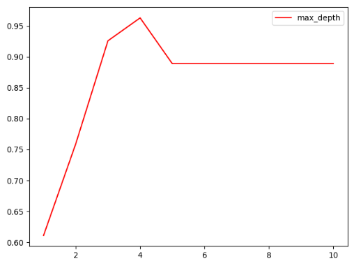
Description Max_ When depth is 4, the effect is the best.

Target weight parameter class_ weight & min_ weight_ fraction_ leaf

Imagine this situation: when the bank wants to judge whether "a person who has a credit card will default", that is, the proportion of yes vs no (1%: 99%). In this case, there is a sample imbalance. At this time, it is necessary to adjust its target weight parameters.

Use class_ The weight parameter balances the sample labels, gives more weight to a small number of labels, makes the model more inclined to a few classes, and models in the direction of capturing a few classes. This parameter defaults to None. This mode means that the same weight is automatically given to all labels in the dataset.

With the weight, the sample size is no longer simply the number of records, but is affected by the input weight. Therefore, pruning needs to be combined at this time_ weight_ fraction_ Leaf is used as a weight based pruning parameter.

Important attributes and interfaces

1. (mentioned above) feature_importances_
Be able to view the importance of each feature to the model
Note the underline that follows_ Cannot be omitted

2.apply
Returns the index of the leaf node where each test sample is located

clf.apply(Xtest)

3.predict returns the classification / regression results of each test sample

clf.predict(Xtest)

Supplement of other contents

The classification tree is not good at ring data, and the nearest neighbor algorithm, RBF support vector machine and Gaussian process are the best at moon data; The nearest neighbor algorithm and Gaussian process are the best at ring data; Naive Bayes, neural networks and random forests are the best at halving data.

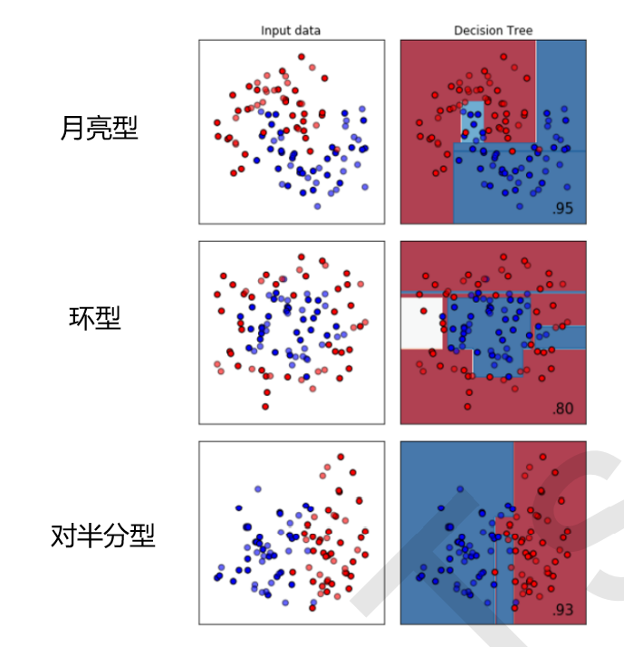
The above is the result of the classification tree. You can see a piece of white on the left of the ring data, indicating that the classification effect is not good.