1. Introduction to sklearn
Scikit learn (sklearn) is a common third-party module in machine learning. It encapsulates common machine learning methods, including regression, dimension reduction, classification, clustering and other methods. When we face the problem of machine learning, we can choose the corresponding method according to the figure below. Sklearn has the following features: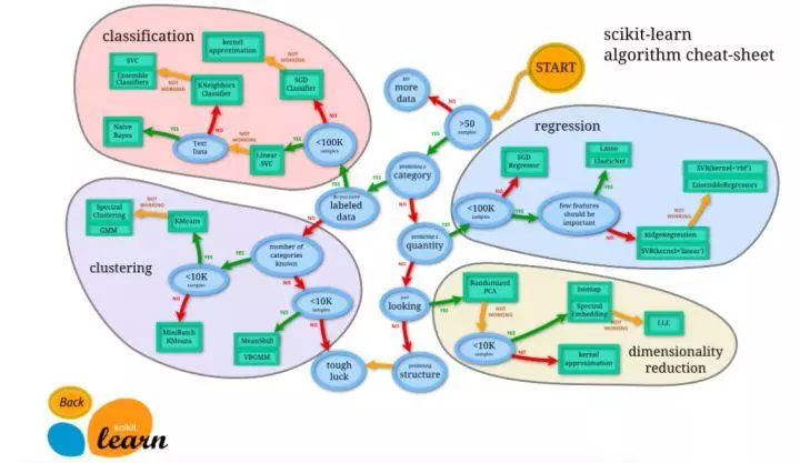

Simple and efficient data mining and analysis tools
Enable everyone to reuse in a complex environment
Build NumPy, Scipy and MatPlotLib
image
2.Sklearn installation
Sklearn installation requires python (> = 2.7 or > = 3.3), NumPy (> = 1.8.2), SciPy (> = 0.13.3). If NumPy and SciPy are already installed, install scikit learn using PIP install - u scikit learn.

3.Sklearn general learning mode
There are many machine learning methods in sklearn, but they are almost the same. We will introduce the general learning mode of sklearn here. Firstly, introduce the data to be trained. Sklearn comes with some data sets, which can also be constructed by corresponding methods. 4. In sklearn data sets, we will introduce how to construct data. Then choose the corresponding machine learning method for training. During the training process, you can adjust the parameters through some skills, so that the learning accuracy is higher. After the Model training, we can predict the new data, and then we can show the data intuitively by means of MatPlotLib and other methods. In addition, we can save the trained Model, which is convenient to move to other platforms without retraining.

from sklearn import datasets#Introducing data sets, sklearn contains many data sets
from sklearn.model_selection import train_test_split#Divide data into test set and training set
from sklearn.neighbors import KNeighborsClassifier#Training data by neighboring points

###Import data###
iris=datasets.load_iris()#Iris iris data is introduced. Iris data contains 4 characteristic variables
iris_X=iris.data#Characteristic variable
iris_y=iris.target#target value
X_train,X_test,y_train,y_test=train_test_split(iris_X,iris_y,test_size=0.3)#Use train test split to separate training set and test set, with test size accounting for 30%
print(y_train)#We can see that the eigenvalues of training data are divided into three categories
'''
[0 0 0 0 0 0 0 0 0 0 0 0 0 0 0 0 0 0 0 0 0 0 0 0 0 0 0 0 0 0 0 0 0 0 0 0 0
 0 0 0 0 0 0 0 0 0 0 0 0 0 1 1 1 1 1 1 1 1 1 1 1 1 1 1 1 1 1 1 1 1 1 1 1 1
 1 1 1 1 1 1 1 1 1 1 1 1 1 1 1 1 1 1 1 1 1 1 1 1 1 1 2 2 2 2 2 2 2 2 2 2 2
 2 2 2 2 2 2 2 2 2 2 2 2 2 2 2 2 2 2 2 2 2 2 2 2 2 2 2 2 2 2 2 2 2 2 2 2 2
 2 2]
 '''

###Training data###
knn=KNeighborsClassifier()#Introducing training methods
knn.fit(X_train,y_train)#Filling test data for training

###Forecast data###
print(knn.predict(X_test))#Predicted eigenvalue
'''
[1 1 1 0 2 2 1 1 1 0 0 0 2 2 0 1 2 2 0 1 0 0 0 0 0 0 2 1 0 0 0 1 0 2 0 2 0
 1 2 1 0 0 1 0 2]
'''
print(y_test)#True eigenvalue
'''
[1 1 1 0 1 2 1 1 1 0 0 0 2 2 0 1 2 2 0 1 0 0 0 0 0 0 2 1 0 0 0 1 0 2 0 2 0
 1 2 1 0 0 1 0 2]
'''

4.Sklearn datasets
Sklearn provides some standard data, so we don't have to look for data from other websites for training. For example, the load? Iris data used for training above can easily return data characteristic variables and target values. In addition to introducing data, we can also import images through load? Sample? Images().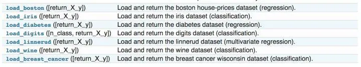

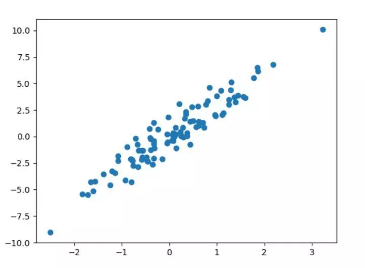
In addition to some data provided by sklearn, we can also construct some data ourselves to help us learn.

from sklearn import datasets#Import data set
#Various parameters of the structure can be adjusted according to your own needs
X,y=datasets.make_regression(n_samples=100,n_features=1,n_targets=1,noise=1)

###Draw constructed data###
import matplotlib.pyplot as plt
plt.figure()
plt.scatter(X,y)
plt.show()

5. Properties and functions of sklearn model
After the data training, we can get the model. We can get the corresponding attributes and functions according to different models, and output them to get intuitive results. If the linear function y=0.3x+1 is obtained after the linear regression training, we can get the coefficient of the model as 0.3 through ﹣ coef ﹣ and the intercept of the model as 1 through ﹣ intercept ﹣.

from sklearn import datasets
from sklearn.linear_model import LinearRegression#Introducing linear regression model

###Import data###
load_data=datasets.load_boston()
data_X=load_data.data
data_y=load_data.target
print(data_X.shape)
#(506, 13) data × 13 characteristic variables in total

###Training data###
model=LinearRegression()
model.fit(data_X,data_y)
model.predict(data_X[:4,:])#Forecast top 4 data

###Properties and functions###
print(model.coef_)
'''
[ -1.07170557e-01   4.63952195e-02   2.08602395e-02   2.68856140e+00
  -1.77957587e+01   3.80475246e+00   7.51061703e-04  -1.47575880e+00
   3.05655038e-01  -1.23293463e-02  -9.53463555e-01   9.39251272e-03
  -5.25466633e-01]
'''
print(model.intercept_)
#36.4911032804
print(model.get_params())#Get the parameters of the model
#{'copy_X': True, 'normalize': False, 'n_jobs': 1, 'fit_intercept': True}
print(model.score(data_X,data_y))#Score training
#0.740607742865

6.Sklearn data preprocessing
The standardization of data sets is a common requirement for most machine learning algorithms. If a single feature is not more or less close to the standard normal distribution, it may not perform well in the project. In practice, we often ignore the distribution shape of the feature, directly remove the mean value to centralize a feature, and then divide by the standard deviation of non constant features to scale.

For example, in many learning algorithms, the basis of objective function is to assume that all features are zero mean and have variance of the same order (such as radial basis function, support vector machine, L1L2 regularization term, etc.). If the variance of a feature is several orders of magnitude larger than that of other features, it will occupy a dominant position in the learning algorithm, resulting in that the learner can not learn from other features as we expect. For example, we can Scale the data through Scale to achieve the goal of standardization.

from sklearn import preprocessing
import numpy as np
a=np.array([[10,2.7,3.6],
            [-100,5,-2],
            [120,20,40]],dtype=np.float64)
print(a)
print(preprocessing.scale(a))#Reduce the difference between values
'''
[[  10\.     2.7    3.6]
 [-100\.     5\.    -2\. ]
 [ 120\.    20\.    40
[[ 0\.         -0.85170713 -0.55138018]
 [-1.22474487 -0.55187146 -0.852133  ]
 [ 1.22474487  1.40357859  1.40351318]]
'''

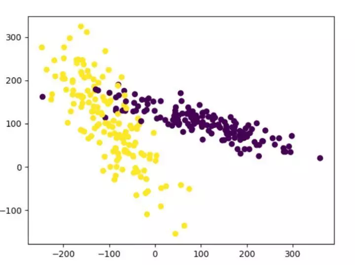
Let's look at the difference between the pre-treatment and the pre-treatment. The model score before the pre-treatment is 0.511111111111, and the model score after the pre-treatment is 0.933333333. We can see that the pre-treatment greatly improves the model score.

from sklearn.model_selection import train_test_split
from sklearn.datasets.samples_generator import make_classification
from sklearn.svm import SVC
import matplotlib.pyplot as plt

###The generated data is shown in the figure below###
plt.figure
X,y=make_classification(n_samples=300,n_features=2,n_redundant=0,n_informative=2,             random_state=22,n_clusters_per_class=1,scale=100)
plt.scatter(X[:,0],X[:,1],c=y)
plt.show()

###utilize minmax Method to standardize data###
X=preprocessing.minmax_scale(X)#Feature [range = (- 1,1) reset range can be set
X_train,X_test,y_train,y_test=train_test_split(X,y,test_size=0.3)
clf=SVC()
clf.fit(X_train,y_train)
print(clf.score(X_test,y_test))
#0.933333333333
#Before normalization, our training score was 0.511111111111, and after normalization, it was 0.933333333, which greatly improved the accuracy

7. Cross validation
The basic idea of cross validation is to group the original data, one as training set to train the model, the other as test set to evaluate the model. Cross validation is used to evaluate the prediction performance of the model, especially the performance of the trained model on the new data, which can reduce the over fitting to a certain extent. It can also obtain as much effective information as possible from the limited data.

In machine learning task, after getting the data, we will first divide the original data set into three parts: training set, verification set and test set. The training set is used to train the model, the validation set is used to select and configure the parameters of the model, and the test set is unknown data for the model, which is used to evaluate the generalization ability of the model. Different partition will result in different final models.

In the past, we directly split the data into 70% of training data and test data. Now we use K-fold cross validation to split the data, first divide the data into five groups, and then select different data from the five groups for training.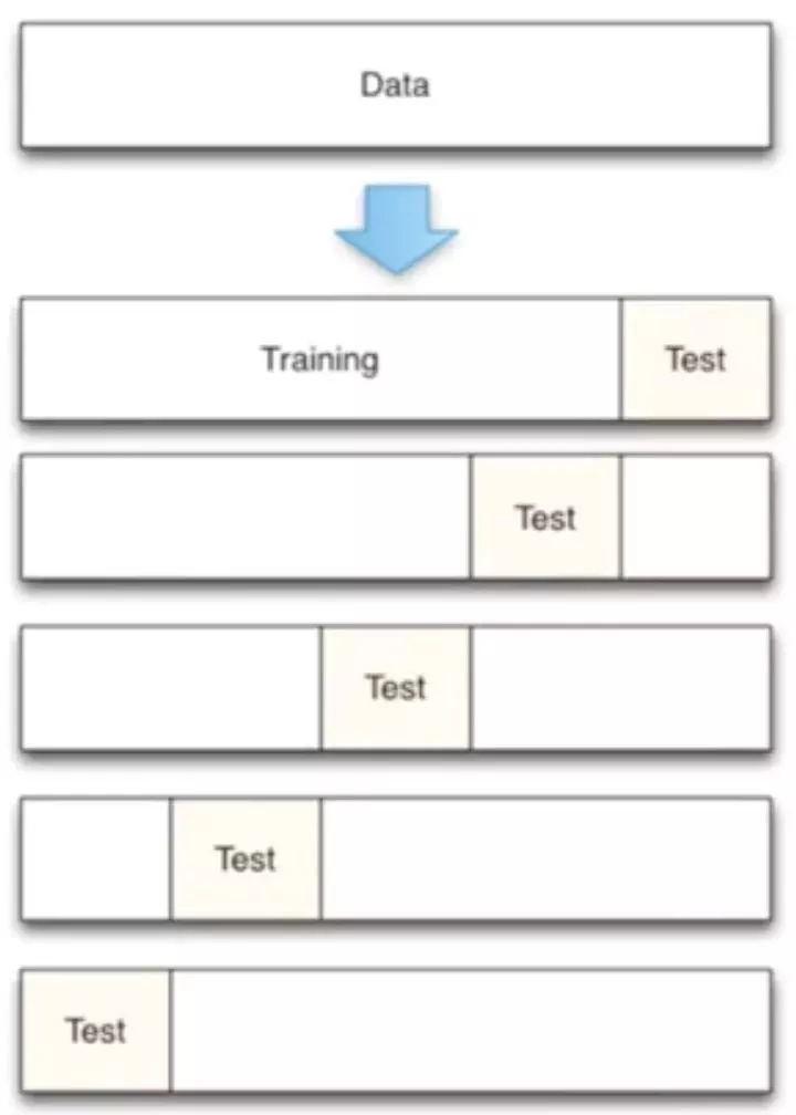

from sklearn.datasets import load_iris
from sklearn.model_selection import train_test_split
from sklearn.neighbors import KNeighborsClassifier

###Import data###
iris=load_iris()
X=iris.data
y=iris.target

###Training data###
X_train,X_test,y_train,y_test=train_test_split(X,y,test_size=0.3)
#Introduce cross validation, and divide the data into 5 groups for training
from sklearn.model_selection import cross_val_score
knn=KNeighborsClassifier(n_neighbors=5)#Select 5 adjacent points
scores=cross_val_score(knn,X,y,cv=5,scoring='accuracy')#Scoring method is accuracy
print(scores)#Scoring results of each group
#[0.96666667 1 \. 0.93333333 0.96666667 1 \.] 5 sets of data
print(scores.mean())#Average score results
#0.973333333333

So whether n ﹐ neighbor = 5 is the best? Let's adjust the parameters to see the final training score of the model.

from sklearn import datasets
from sklearn.model_selection import train_test_split
from sklearn.neighbors import KNeighborsClassifier
from sklearn.model_selection import cross_val_score#Introduce cross validation
import  matplotlib.pyplot as plt
###Import data###
iris=datasets.load_iris()
X=iris.data
y=iris.target
###Set up n_neighbors Values of 1 to 30,See the training score through drawing###
k_range=range(1,31)
k_score=[]
for k in k_range:
    knn=KNeighborsClassifier(n_neighbors=k)
    scores=cross_val_score(knn,X,y,cv=10,scoring='accuracy')#for classfication
    k_score.append(loss.mean())
plt.figure()
plt.plot(k_range,k_score)
plt.xlabel('Value of k for KNN')
plt.ylabel('CrossValidation accuracy')
plt.show()
#K over assembly brings over fitting problem, we can choose the value between 12-18

We can see that the score of n ﹣ neighbor is relatively high between 12-18. In the actual project, we can choose different parameters in this way. In addition, we can choose 2-fold cross validation, leave one out cross validation and other methods to segment data, and compare different methods and parameters to get the optimal results.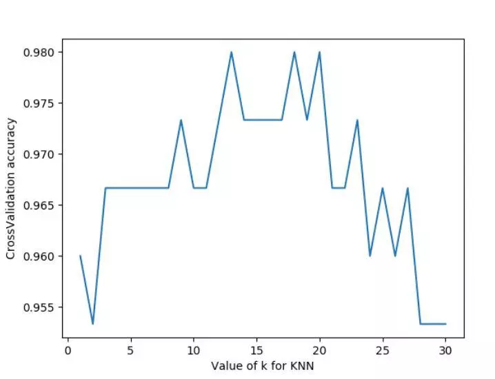

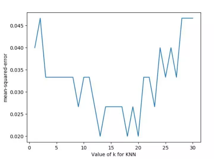
Let's change the part of the loop in the above code, and change the scoring function to neg? Mean? Squared? Error to get the loss function for different parameters.

for k in k_range:
    knn=KNeighborsClassifier(n_neighbors=k)
    loss=-cross_val_score(knn,X,y,cv=10,scoring='neg_mean_squared_error')# for regression
    k_score.append(loss.mean())

8. Over fitting
What is an over fitting problem? For example, in the following picture, the black line can well classify the red point and the blue point, but in the process of machine learning, the model is too tangled with accuracy, which results in the green line. Then in the process of predicting the result of test data set, a lot of time will be wasted and the accuracy is not very good.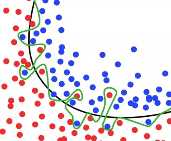

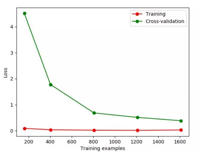
Let's first give an example of how to distinguish the overfitting problem. The learning curve in sklearn.learning'curve can directly see the progress of Model learning, and the comparison shows whether there is any fitting.

from sklearn.model_selection import learning_curve
from sklearn.datasets import load_digits
from sklearn.svm import SVC
import matplotlib.pyplot as plt
import numpy as np

#Import data
digits=load_digits()
X=digits.data
y=digits.target

#Train? Size means to record a certain step in the learning process, such as at 10%, 25% In the process of
train_size,train_loss,test_loss=learning_curve(
SVC(gamma=0.1),X,y,cv=10,scoring='neg_mean_squared_error',
train_sizes=[0.1,0.25,0.5,0.75,1]
)
train_loss_mean=-np.mean(train_loss,axis=1)
test_loss_mean=-np.mean(test_loss,axis=1)

plt.figure()
#Print out every step
plt.plot(train_size,train_loss_mean,'o-',color='r',label='Training')
plt.plot(train_size,test_loss_mean,'o-',color='g',label='Cross-validation')
plt.legend('best')
plt.show()

If we change the value of gamma, we change the Loss function. The Loss function stays at about 10, at this time, we can see the over fitting intuitively.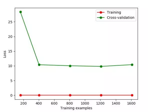

Next, we modify the gamma parameter to correct the over fitting problem.

from sklearn.model_selection import  validation_curve#Change learning curve to validation curve
from sklearn.datasets import load_digits
from sklearn.svm import SVC
import matplotlib.pyplot as plt
import numpy as np
#Import data
digits=load_digits()
X=digits.data
y=digits.target

#Change param to observe the Loss function
param_range=np.logspace(-6,-2.3,5)
train_loss,test_loss=validation_curve(
    SVC(),X,y,param_name='gamma',param_range=param_range,cv=10,
    scoring='neg_mean_squared_error'
)
train_loss_mean=-np.mean(train_loss,axis=1)
test_loss_mean=-np.mean(test_loss,axis=1)

plt.figure()
plt.plot(param_range,train_loss_mean,'o-',color='r',label='Training')
plt.plot(param_range,test_loss_mean,'o-',color='g',label='Cross-validation')
plt.xlabel('gamma')
plt.ylabel('loss')
plt.legend(loc='best')
plt.show()

We can see the change of Loss function by changing different gamma values. As can be seen from the figure, if the gamma value is greater than 0.001, there will be a fitting problem. Then when we build the model, the gamma parameter should be set less than 0.001.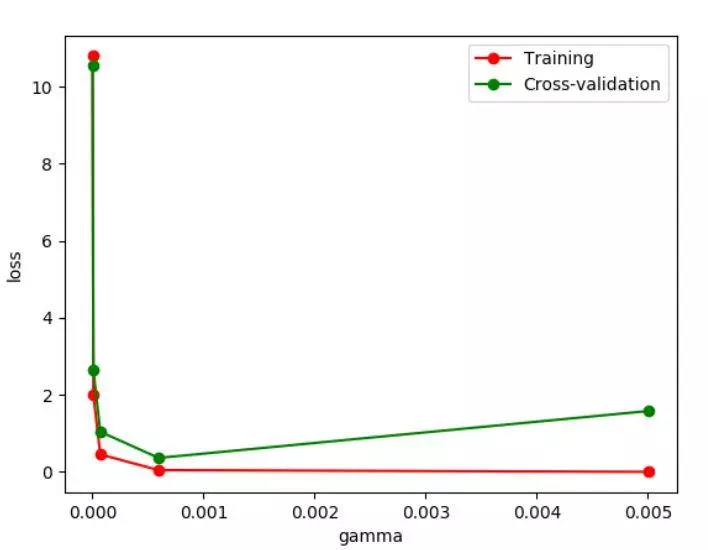

9. Save model
We spend a long time to train the data, adjust the parameters and get the optimal model. But if we change the platform, we need to retrain the data and modify the parameters to get the model, which will be a waste of time. At this point, we can save the model first, and then we can easily migrate the model.

from sklearn import svm
from sklearn import datasets

#Importing and training data
iris=datasets.load_iris()
X,y=iris.data,iris.target
clf=svm.SVC()
clf.fit(X,y)

#Introduce the storage module of sklearn
from sklearn.externals import joblib
#Save model
joblib.dump(clf,'sklearn_save/clf.pkl')

#Reload the model. The model can only be loaded after it is saved once
clf3=joblib.load('sklearn_save/clf.pkl')
print(clf3.predict(X[0:1]))
#Storing model can get previous results faster