0. Preface

After understanding the principle and process of SLAM, individuals often wonder how to design and write a set of SLAM framework that can meet our needs from scratch. The author believes that Ceres, Eigen, Sophus and G2O function libraries cannot be avoided, especially Ceres function libraries are widely used in the optimization of laser SLAM and V-SLAM. The author respectively from Ceres and Eigen The two functions are deeply analyzed. This article mainly expounds the G2O function library in detail to facilitate your subsequent development.

1.G2O example

Compared with Ceres, G2O function library is relatively complex, but it has a wider range of applications and can solve more complex relocation problems. Ceres library is used to solve the general least squares problem, define the optimization problem, and set some options, which can be solved through Ceres. Graph optimization is a way to express the optimization problem as a graph. The graph here is a graph in the sense of graph theory. A graph consists of several vertices and edges connected to them. Here, we use vertices to represent optimization variables and edges to represent error terms.

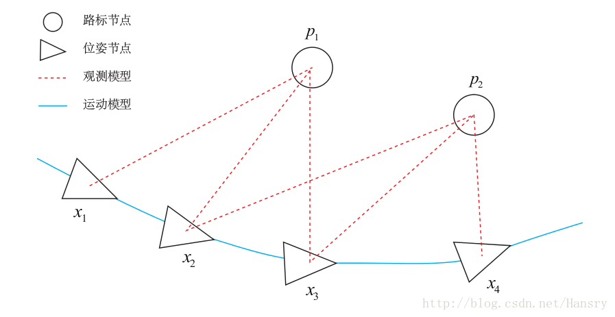
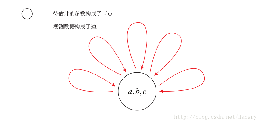
In order to use g2o, we must first abstract the curve fitting problem into graph optimization. In this process, just remember that the node is the optimization variable and the edge is the error term. The graph optimization problem of curve fitting can be drawn in the following form:

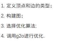
G2O is mathematically divided into four solving steps:

The reaction in the procedure is:

1. Create a linear solver, LinearSolver.
2. Create a BlockSolver and initialize it with the linear solver defined above.
3. Create a total solver solver, select one from GN/LM/DogLeg as the iteration strategy, and then initialize it with the block solver BlockSolver mentioned above.
4. The core of graph creation Optimization: sparse optimizer.
5. Define the vertices and edges of the graph and add them to SparseOptimizer.
6. Set the optimization parameters and start the optimization.

#include <iostream>
#include <g2o/core/base_vertex.h>
#include <g2o/core/base_unary_edge.h>
#include <g2o/core/block_solver.h>
#include <g2o/core/optimization_algorithm_levenberg.h>
#include <g2o/core/optimization_algorithm_gauss_newton.h>
#include <g2o/core/optimization_algorithm_dogleg.h>
#include <g2o/solvers/dense/linear_solver_dense.h>
#include <Eigen/Core>
#include <opencv2/core/core.hpp>
#include <cmath>
#include <chrono>
using namespace std; 

// Vertex and template parameters of curve model: optimization variable dimension and data type (here is user-defined fixed point, please refer to the point definition below for details)
class CurveFittingVertex: public g2o::BaseVertex<3, Eigen::Vector3d>
{
public:
    EIGEN_MAKE_ALIGNED_OPERATOR_NEW// byte alignment 
    virtual void setToOriginImpl() // Reset to set the original value of the optimized variable 
    {
        _estimate << 0,0,0;
    }
    
    virtual void oplusImpl( const double* update ) // to update
    {
        _estimate += Eigen::Vector3d(update);//update cast type to Vector3d
    }
    // Save and read: leave blank
    virtual bool read( istream& in ) {}
    virtual bool write( ostream& out ) const {}
};

// Error model template parameters: observation dimension, type, connection vertex type
class CurveFittingEdge: public g2o::BaseUnaryEdge<1,double,CurveFittingVertex>
{
public:
    EIGEN_MAKE_ALIGNED_OPERATOR_NEW
    CurveFittingEdge( double x ): BaseUnaryEdge(), _x(x) {}
    // Calculation curve model error
    void computeError()
    {
        const CurveFittingVertex* v = static_cast<const CurveFittingVertex*> (_vertices[0]);
        const Eigen::Vector3d abc = v->estimate();
        _error(0,0) = _measurement - std::exp( abc(0,0)*_x*_x + abc(1,0)*_x + abc(2,0) ) ;
    }
    virtual bool read( istream& in ) {}
    virtual bool write( ostream& out ) const {}
public:
    double _x;  // x value, y value is_ measurement
};

int main( int argc, char** argv )
{
    double a=1.0, b=2.0, c=1.0;         // True parameter value
    int N=100;                          // data point
    double w_sigma=1.0;                 // Noise Sigma value
    cv::RNG rng;                        // OpenCV random number generator
    double abc[3] = {0,0,0};            // Estimation of abc parameters

    vector<double> x_data, y_data;      // data
    
    cout<<"generating data: "<<endl;
    for ( int i=0; i<N; i++ )
    {
        double x = i/100.0;
        x_data.push_back ( x );
        y_data.push_back (
            exp ( a*x*x + b*x + c ) + rng.gaussian ( w_sigma )
        );
        cout<<x_data[i]<<" "<<y_data[i]<<endl;
    }
    
    // To optimize the construction diagram, set g2o first
    typedef g2o::BlockSolver< g2o::BlockSolverTraits<3,1> > Block;  // The optimization variable dimension of each error item is 3 and the error value dimension is 1
    Block::LinearSolverType* linearSolver = new g2o::LinearSolverDense<Block::PoseMatrixType>(); // Linear equation solver. Step 1: create a linear solver, LinearSolver.
    Block* solver_ptr = new Block( linearSolver );      // Matrix block solver. Step 2: create BlockSolver and initialize it with the linear solver defined above.
    // Gradient descent method, selected from GN, LM, DogLeg
    g2o::OptimizationAlgorithmLevenberg* solver = new g2o::OptimizationAlgorithmLevenberg( solver_ptr );//Step 3: create BlockSolver and initialize it with the linear solver defined above.
    // g2o::OptimizationAlgorithmGaussNewton* solver = new g2o::OptimizationAlgorithmGaussNewton( solver_ptr );
    // g2o::OptimizationAlgorithmDogleg* solver = new g2o::OptimizationAlgorithmDogleg( solver_ptr );
    g2o::SparseOptimizer optimizer;     // Figure model. Step 4: create the core of graph optimization: sparse optimizer.
    optimizer.setAlgorithm( solver );   // Set up solver
    optimizer.setVerbose( true );       // Open debug output
    
    // Add vertices to the graph. Step 5: define the vertex and edge HyperGraph of the graph and add it to SparseOptimizer.
    CurveFittingVertex* v = new CurveFittingVertex();
    v->setEstimate( Eigen::Vector3d(0,0,0) );
    v->setId(0);
    optimizer.addVertex( v );
    
    // Add edges to the graph
    for ( int i=0; i<N; i++ )
    {
        CurveFittingEdge* edge = new CurveFittingEdge( x_data[i] );
        edge->setId(i);
        edge->setVertex( 0, v );                // Set connected vertices
        edge->setMeasurement( y_data[i] );      // Observed value
        edge->setInformation( Eigen::Matrix<double,1,1>::Identity()*1/(w_sigma*w_sigma) ); // Information matrix: inverse of covariance matrix
        optimizer.addEdge( edge );
    }
    
    // Perform optimization. Step 6: set the optimization parameters and start the optimization.
    cout<<"start optimization"<<endl;
    chrono::steady_clock::time_point t1 = chrono::steady_clock::now();
    optimizer.initializeOptimization();
    optimizer.optimize(100);
    chrono::steady_clock::time_point t2 = chrono::steady_clock::now();
    chrono::duration<double> time_used = chrono::duration_cast<chrono::duration<double>>( t2-t1 );
    cout<<"solve time cost = "<<time_used.count()<<" seconds. "<<endl;
    
    // Output optimization value
    Eigen::Vector3d abc_estimate = v->estimate();
    cout<<"estimated model: "<<abc_estimate.transpose()<<endl;
    
    return 0;
}

2. Summary of common g2o functions

As shown in the figure below, this figure reflects the first five steps above

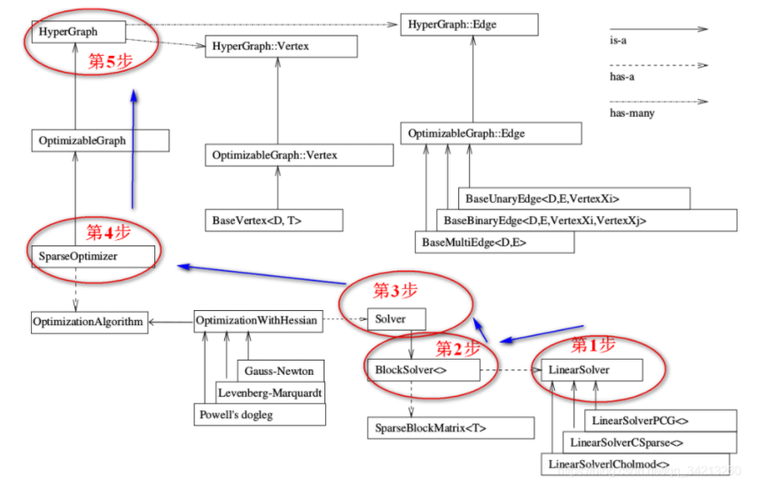
Make a brief introduction to the structural block diagram (pay attention to the meanings of the three arrows in the figure (notes in the upper right corner)):

(1) Core of $\ color{#4285f4}{diagram: the whole g2o framework can be divided into upper and lower parts, and the connection point between the two parts: SparseOpyimizer is the core of the whole g2o.

(2) Looking up, SparseOpyimizer is actually an optimized graph, and thus a HyperGraph.

(3) top spot and edge : \color{#4285f4}{vertices and edges:} Vertices and edges: hypergraphs have many vertices and edges. Vertices are inherited from Base Vertex, i.e. OptimizableGraph::Vertex; The edges can be inherited from BaseUnaryEdge (unilateral), BaseBinaryEdge (bilateral) or BaseMultiEdge (multilateral), which are all called OptimizableGraph::Edge.

(4) match Set S p a r s e O p t i m i z e r of excellent turn count method and seek solution implement : \color{#4285f4}{configure SparseOptimizer's optimization algorithm and Solver:} Configure SparseOptimizer's optimization algorithm and Solver: looking down, SparseOptimizer includes an optimization algorithm part, optimization algorithm, which is implemented through optimization with Hessian. The iterative strategy can be selected from * * Gauss Newton (GN), levernberg Marquardt (LM) and Powell's dogleg * * (GN and LM are commonly used).

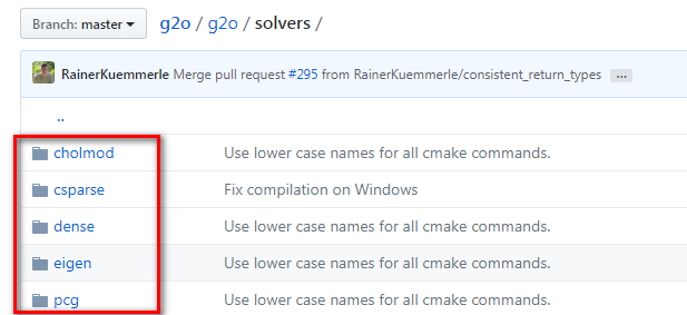
(5) as What seek solution : \color{#4285f4}{how to solve:} How to solve: when solving the optimization algorithm part, the solver is actually composed of BlockSolver. BlockSolver consists of two parts: one is SparseBlockMatrix, which solves sparse matrices (Jacobi and Hesse); The other part is LinearSolver, which is used to solve linear equations to obtain the increment to be solved. Therefore, this part is very important. It can choose the solution method from PCG/CSparse/Choldmod.

2.1 create a linear solver LinearSolver

The form of the incremental equation we require is: H △ X=-b. generally, the method we think of is to find the inverse directly, that is, △ X=-H.inv*b. It seems very simple, but there is a premise that the dimension of H is small. At this time, only the inverse of the matrix can solve the problem. However, when the dimension of H is large, the inversion of matrix is very difficult, and the problem becomes very complex. Similar to Ceres, G2O needs some special methods to inverse the matrix.

... please refer to Gu Yueju