catalogue
6.1 counting and sorting (selection and mastery)
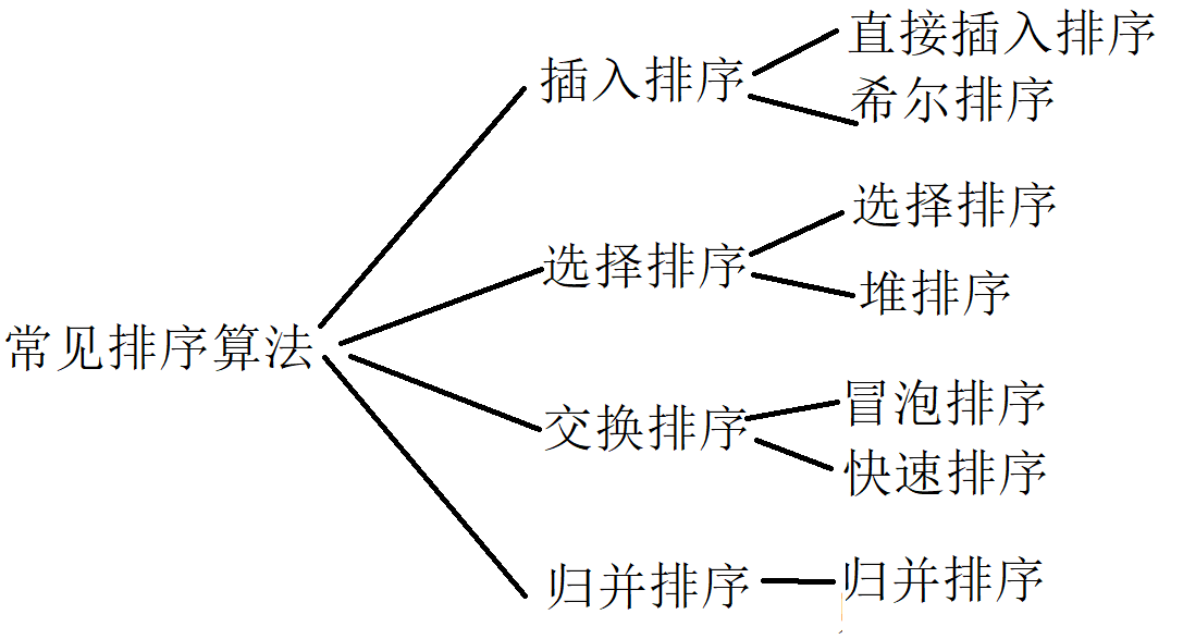
1. Sorting and classification
2. Insert sort
2.1 direct insertion sort
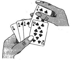
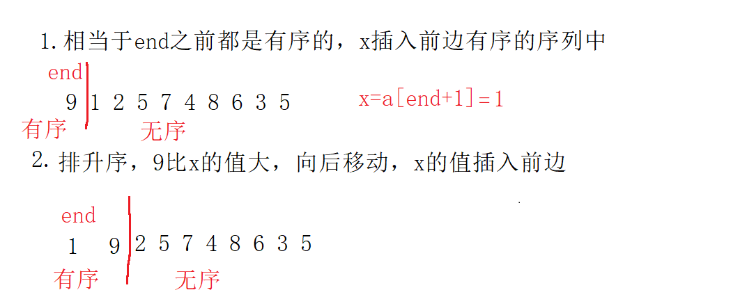
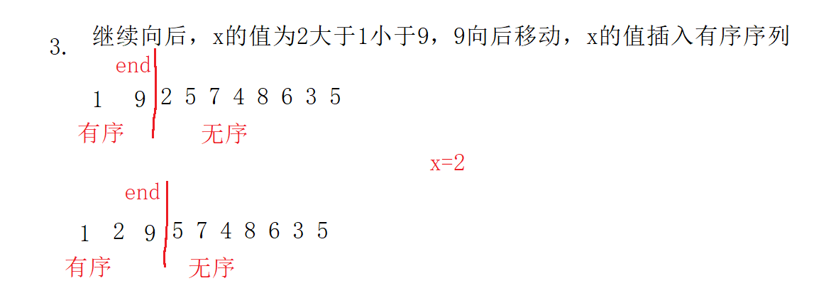
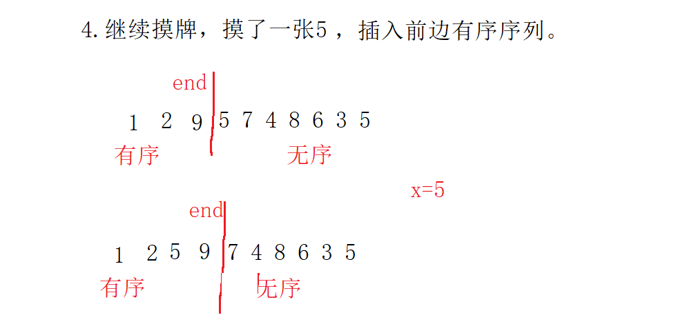
Direct insertion sorting is a simple insertion sorting method. The basic idea is: it is the same as playing poker. See the figure below.
Insert sort code:
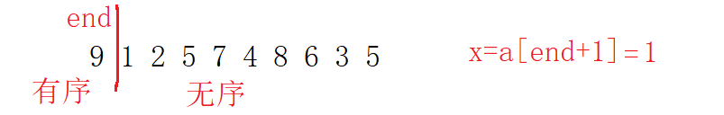
When writing code, you can write the (two data) inside first:
void InsertSort(int* a, int n)
{

	int end = 0;
	int x = a[end + 1];
	while (end>=0)
	{
		if (x < a[end])
		{
			a[end] = a[end + 1];
			end--;
		}
		else
		{
			break;
		}
	}
	a[end + 1] = x;
}
Then control all data:
void InsertSort(int* a, int n)
{
	for (int i = 0; i < n-1; i++)
	{
		int end=i;
		int x = a[end + 1];
		while(end >= 0)
		{
			if ( x < a[end] )
			{
				a[end + 1] = a[end];
				end--;
			}
			else
			{
				break;
			}
		}
		a[end + 1] = x;
	}
}
main.c test code:
int main()
{
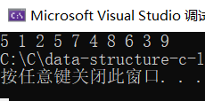
int a[] = {9,1,2,5,7,4,8,6,3,5 };
InsertSort(a,sizeof(a) / sizeof(a[0]));
ArryPrint(a, sizeof(a) / sizeof(a[0]));
return 0;
}result:
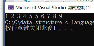
Sorting process:
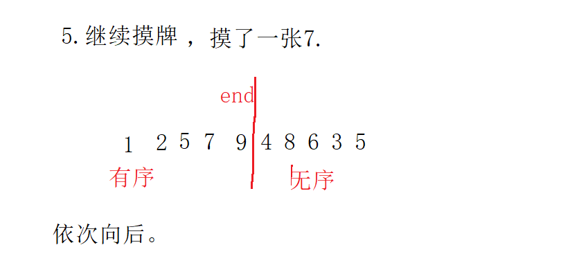
Here's the picture above. Hee hee, steal a lazy!
Insert sort complexity analysis:
Best case: when the data of the array is: 1,2,3,4,5,6,7,8,9. Each data is only compared with the last data, so the complexity is O(N).
Worst case: when the array data is: 9,8,7,6,5,4,3,2,1. 8 compared forward once, 7 compared forward twice, 6 compared forward three times, 1 forward compares N-1, the arithmetic sequence, so the complexity is O(N^2).
2.2. Shell Sort
1. Hill sort is the optimization of direct insertion sort
2. When gap > 1, it is pre sort. The purpose is to make the data of the array close to order, and then let gap==1. The array is close to order, and direct insertion sorting is realized, which is very fast. Because when direct insertion sorting is in order, the complexity is O(N). In this way, the optimization effect can be achieved as a whole.
3. Code implementation:
main. Test code:
int main()
{

	int a[] = {9,1,2,5,7,4,8,6,3,5 };
	ShellSort(a,sizeof(a) / sizeof(a[0]));
	ArryPrint(a, sizeof(a) / sizeof(a[0]));
	return 0;
}
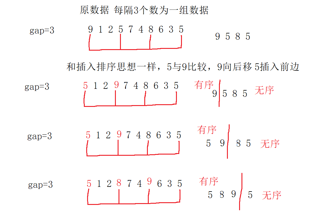
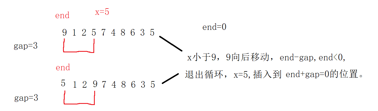
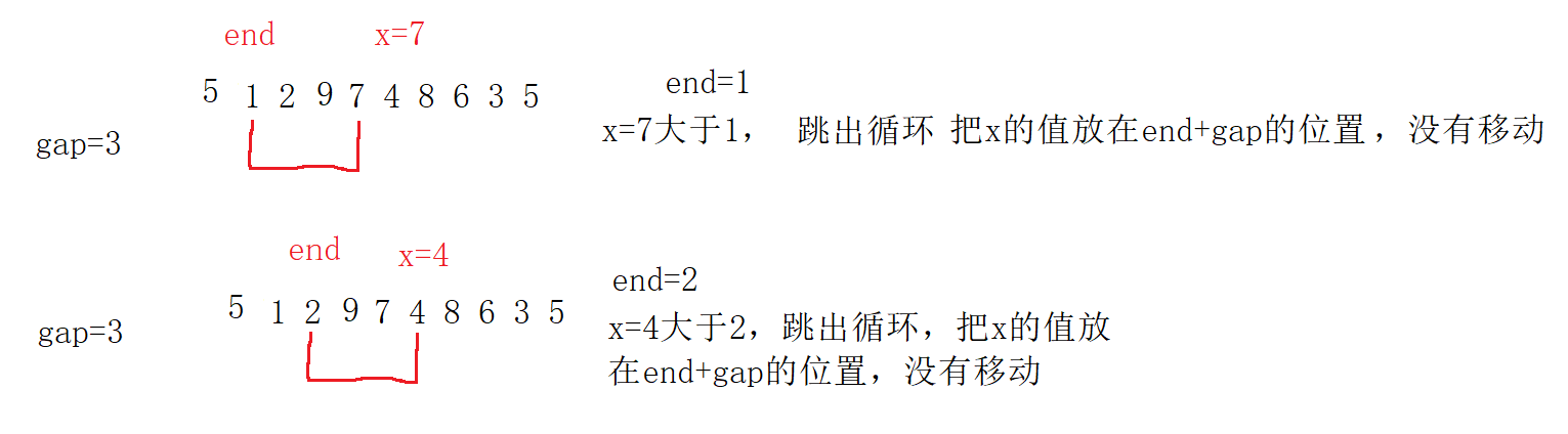
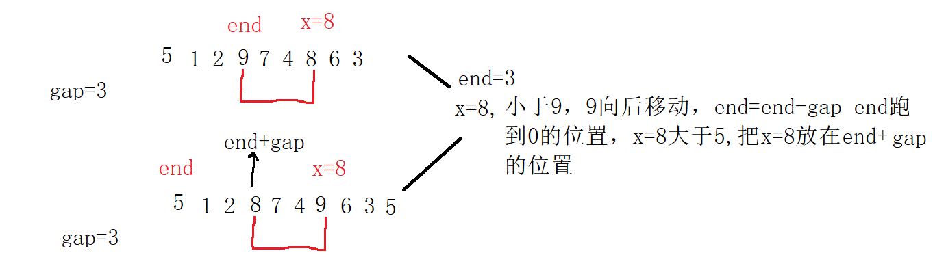
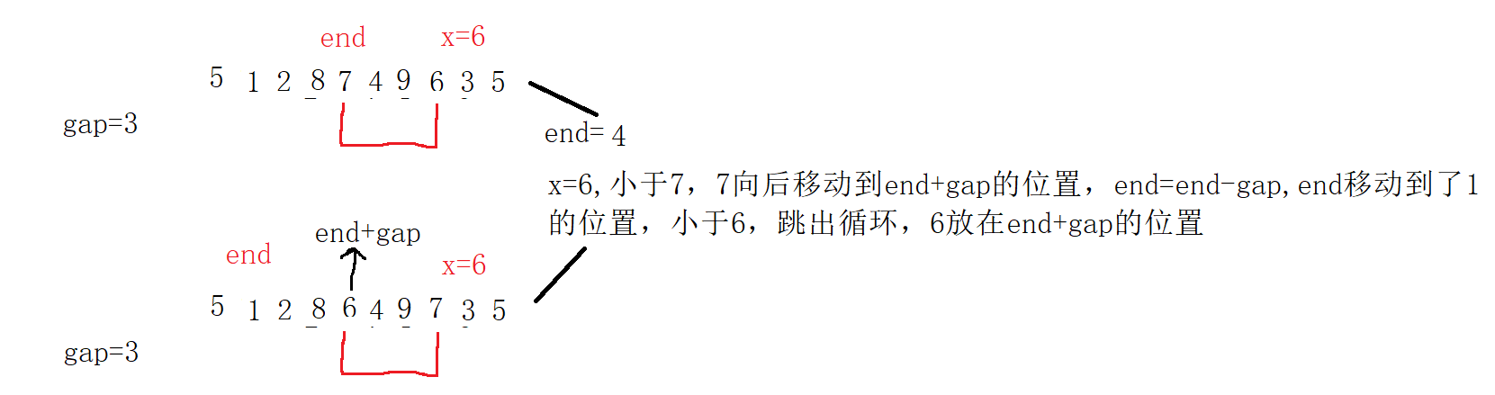
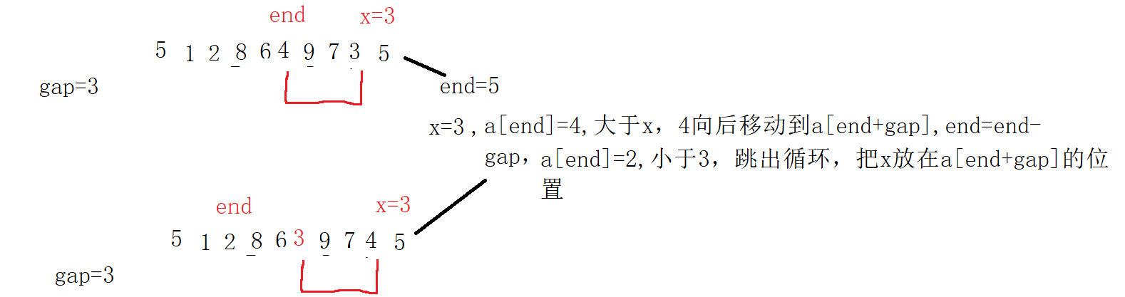
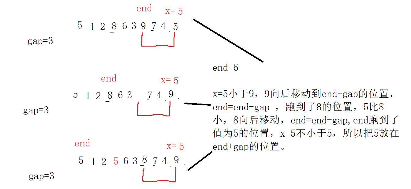
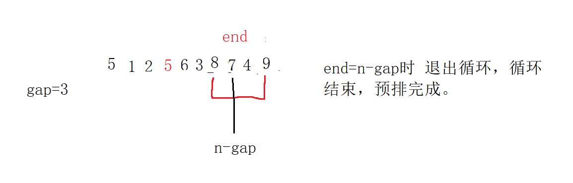
The first step is to write a single group for pre scheduling. The test array data is 9,1,2,5,7,4,8,6,3,5.
void ShellSort(int* a, int n)
{
int gap = 3;
for (int i = 0; i < n - gap; i += gap)
{
int end = i;
int x = a[end + gap];
while (end >= 0)
{
if (a[end] > x)
{
a[end + gap] = a[end];
end -= gap;
}
else
{
break;
}
}
a[end + gap] = x;
}
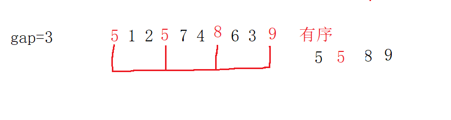
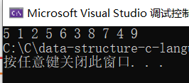
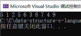
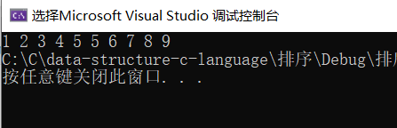
}result:
Process:
The second step is to write the pre sorting of all groups (a total of 3 groups):
void ShellSort(int* a, int n)
{

	int gap = 3;
	for (int j = 0; j < gap; j++)
	{
		for (int i = j; i < n - gap; i += gap)
		{
			int end = i;
			int x = a[end + gap];

			while (end >= 0)
			{
				if (a[end] > x)
				{
					a[end + gap] = a[end];
					end -= gap;
				}
				else
				{
					break;
				}
			}
			a[end + gap] = x;
		}
	}


}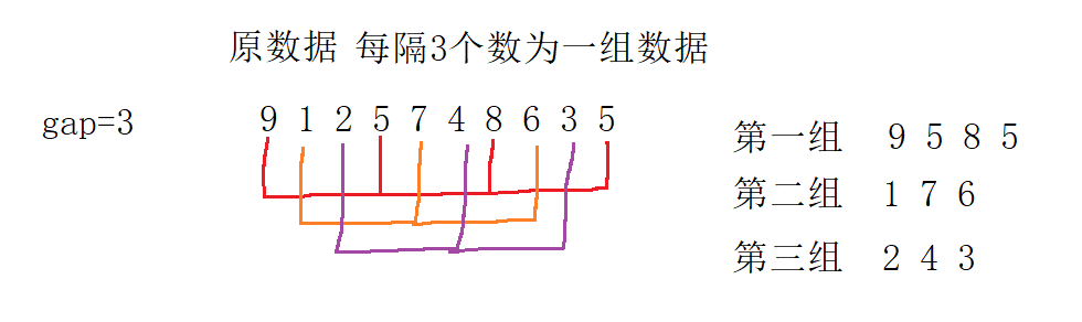
The first group of pre scheduling is completed in the following order: 5 5 8 9
The second group of pre scheduling is completed in the following order: 1 6 7
The third group of pre scheduling is completed in the following order: 2 3 4
Each group is pre sorted, which is the same as that of the single group above. The results are as follows:
Complexity analysis of 3 groups of pre scheduled codes (time):
Best case: each group is ordered, which is equivalent to direct insertion and ordering, and the complexity is O(N). Therefore, the best result of three groups of pre scheduling is O(N).
Worst case: when each group is out of order, the data of each group is about N/gap, and the sorting times of each group are: F(N, gap) = 1 + 2 + 3+ N/gap, the total number of times of the three groups is: F(N, gap)=(1+2+3+...+N/gap)*gap. The smaller the gap, the slower the row. For example, when gap=1, it is a direct insertion sort. The complexity is O(n^2). The slower the row, but the closer it will be to order; When gap is close to N, the faster the row, the less close to order.
4. Optimize multiple groups of sorting codes above:
Multiple groups are arranged together and side by side: one layer of looping modification is missing: for (int i = 0; I < n-gap; I + +)
void ShellSort(int* a, int n)
{
int gap = 3;
for (int i = 0; i < n - gap; i++)
{
int end = i;
int x = a[end + gap];
while (end >= 0)
{
if (a[end] > x)
{
a[end + gap] = a[end];
end -= gap;
}
else
{
break;
}
}
a[end + gap] = x;
}
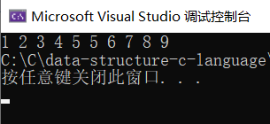
}The improved results are as follows:
The process is:
5. Now start with gap and sort the nearly ordered arrays.
Note: for gap, gap==1 must be guaranteed for the last time, which is equivalent to direct insertion sorting. However, the array has been pre arranged several times, which is close to order, and the complexity is O(N);
void ShellSort(int* a, int n)
{

	int gap = n;
	while (gap > 1)
	{
		gap /= 2;
        //gap=gap/3+1;
		for (int i = 0; i < n - gap; i++)
		{
			int end = i;
			int x = a[end + gap];

			while (end >= 0)
			{
				if (a[end] > x)
				{
					a[end + gap] = a[end];
					end -= gap;
				}
				else
				{
					break;
				}
			}
			a[end + gap] = x;
		}
	}

}
result:

Complexity analysis: gap=gap/2, which is equivalent to the while loop , the complexity of multi group pre scheduling is F(N,gap) = (1+2+3+...+N/gap) * gap. When gap is N/2, the complexity of multi group pre scheduling is (1+2)*N/2, which is approximately equal to O(N), and the worst is O(N). When gap is very small, for example, when it is 1, it is a direct insertion sort. Although it is O(N^2), it is not N^2 here. Because pre scheduling has been carried out for many times, it is close to order, so the complexity is O(N), So the complexity is O(N*). The official gave O(n^1.3). It's hard to understand. Understand O(N*)All right.
3. Select Sorting
3.1 selection and sorting
Basic idea: select the smallest (or largest) element from the data elements to be sorted each time and store it in the actual position of the sequence until all the data elements to be sorted are finished.
void SelectSort(int* a,int n)
{
	int begin = 0;
	int end = n - 1;
	while (begin < end)
	{
		int maxi = begin;
		int mini = begin;

		for (int i = begin; i <= end; i++)
		{
			if (a[i] < a[mini])
			{
				mini = i;
			}

			if (a[i] > a[maxi])
			{
				maxi = i;
			}
		}

		swap(&a[mini], &a[begin]);
		//When the maximum value and begin are in the same position, and then change the mini, the maximum value will be changed away
		if (begin == maxi)
		{
			maxi = mini;
		}
		swap(&a[maxi], &a[end]);
		begin++;
		end--;

	}


}
Test code:
int main()
{

	int a[] = {9,1,2,5,7,4,8,6,3,5 };
	SelectSort(a,sizeof(a) / sizeof(a[0]));
	ArryPrint(a, sizeof(a) / sizeof(a[0]));
	return 0;
}
Results:
Process:
Complexity analysis:
3.2. Heap sort
Heap sort refers to a sort algorithm designed by using the data structure of heap tree (heap). It is a kind of selective sort. It selects data through heap. It should be noted that I love to build a large heap in ascending order and a small heap in descending order.
Heap sort code:
void AdjustUp(int *a ,int child)
{
	int partent = (child - 1) / 2;
	while (child > 0)
	{
		if (a[child] > a[partent])
		{
			swap(&a[child], &a[partent]);
			child=partent;
			partent = (child - 1) / 2;
		}
		else
		{
			break;
		}
	}

}
void AdjustDown(int* a, int n, int partent)
{
	int child = partent * 2 + 1;

	while (child < n)
	{
		if (child + 1 < n && a[child + 1]>a[child] )
		{
			child++;
		}

		if (a[child] > a[partent] )
		{
			swap(&a[partent],&a[child]);
			partent = child;
			child = partent * 2 + 1;
		}
		else
		{
			break;
		}
	}
}


//Heap sort
//Complexity is O(N*logN)
//Use the downward adjustment to build the reactor to O (N), and the remaining N-1 is adjusted to N*logN
void HeapSort(int* a, int n)
{

	for (int i = 1; i < n; i++)
	{
		AdjustUp(a,i);//Heap building is O(N*logN)
	}
	//Build the heap first, arrange the heap in ascending order, and adjust it downward
	/*int i = 0;
	for (i = (n - 1 - 1) / 2; i >= 0; i--)
	{
		AdjustDown(a,n,i);//Build heap is O(N)
	}*/

	for (int end = n-1; end > 0; end--)
	{
		swap(&a[0],&a[end]);
		AdjustDown(a, end, 0);
	}


}
main.c test code:
int main()
{

	int a[] = {9,1,2,5,7,4,8,6,3,5 };
	HeapSort(a,sizeof(a) / sizeof(a[0]));
	ArryPrint(a, sizeof(a) / sizeof(a[0]));
	return 0;
}
Results:
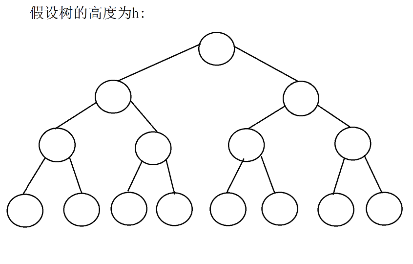
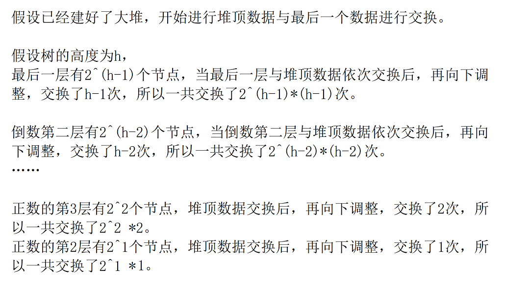
The process of heap sorting has been written in the binary tree! Steal a lazy..
Supplementary analysis on the complexity of heap sorting: the use of downward adjustment is O(N) has been introduced in the binary tree. Here, the complexity of downward and upward adjustment is mainly supplemented.
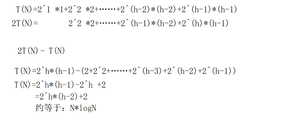
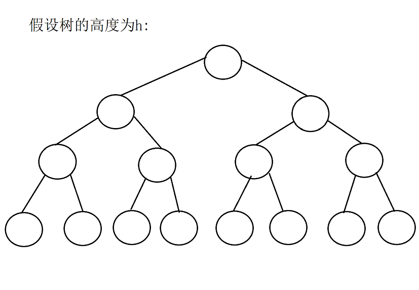
1. Mainly prove why it is O(N*logN). Statement: logN==, steal a lazy!!.
//In heap sorting, the complexity here is O(N*logN)
for (int end = n-1; end > 0; end--)
	{
		swap(&a[0],&a[end]);
		AdjustDown(a, end, 0);
	}
2. To demonstrate the complexity of using upward adjustment heap building.
for (int i = 1; i < n; i++)
	{
		AdjustUp(a,i);O(N*logN)
	}
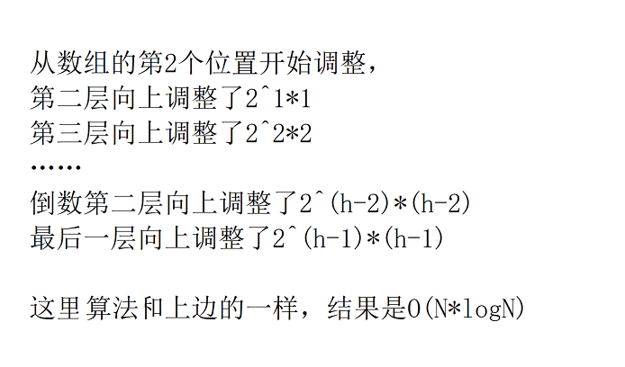
Therefore, the upward adjustment of O(N*logN) is not as good as the downward adjustment, so the downward adjustment of O(N) is generally used for heap building. The overall heap sorting complexity is O(N*logN).
4. Exchange sorting
4.1 bubble sorting
Bubble sorting is familiar. It is optimized in sequence here, that is, in the case of order, without exchange, flag=0 will jump out of the loop in advance;
//The first number is compared n-1 times, and the second number is compared n-2 times,.... The last number is compared once
//Worst complexity O (N^2)
//The worst after improvement: O (N), close to order, or order

void BubbleSort(int *a ,int n)
{

	for (int j = 0; j < n; j++)
	{
		int flag = 0;
		for (int i = 0; i < n -1-j; i++)
		{
			if (a[i] > a[i + 1])
			{
				swap(&a[i], &a[i + 1]);
				flag = 1;
			}

		}
		if (flag == 0)
		{
			break;
		}
	}
}
Complexity analysis: bubble sorting. In the case of disorder, the complexity is O(N^2). If it is close to order, for example, the complexity of bubble sorting is O(N) times 1, 2, 3, 4, 5, 6, 8 and 7.
Compare selection sort with bubble sort and direct insertion sort:
First, analyze the worst case. The complexity of the three sorts is O(N^2), and they need to be compared from the beginning. For example, 2, 5, 1, 3, 4, 6, at this time:
Selection sorting is to start from a number, select the maximum and minimum from beginning to end, and put them on both sides, n-1, n-3, N-5, N-7 1, equal difference sequence, so it is O(N^2)
Insert sorting, you need to insert forward from the first number, 1,2,3,4,5 N-1 is also an equal difference sequence, O(N^2)
Bubble sorting requires a round of upward selection of the maximum number. The first time is n-1, n-2, n-3 1. Arithmetic sequence, O(N^2)
Secondly, when it is close to order, such as 1, 2, 3, 4, 6, 5, at this time:
The worst or best sorting is O(N^2). In any case, you need to traverse from scratch to select the maximum and minimum, and put them on both sides, n-1, n-3, N-5 1.
When the insertion sort is close to order, if it is completely ordered, traverse it again, that is, compare N-1 times, one is not ordered, 5 compare it twice, and compare N-1+2=N+1.
Bubble sorting: after traversing for the first time, bubble 6, compare it N-1 times, and then traverse it again. Only then can we know that it is an ordered array. The cycle ends in advance, N-1+N-1=2N-2 times.
Summary: in the case of near order, the selection sort is the worst sort, the bubble sort is moderate, and the best is the insertion sort.
4.2 quick sort
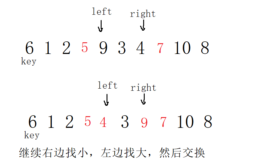
The first step is to write a single trip first: there are three methods for a single trip: 1 Single trip of hoare version 2 Single trip of excavation method 3 Single pass of front and back pointer method
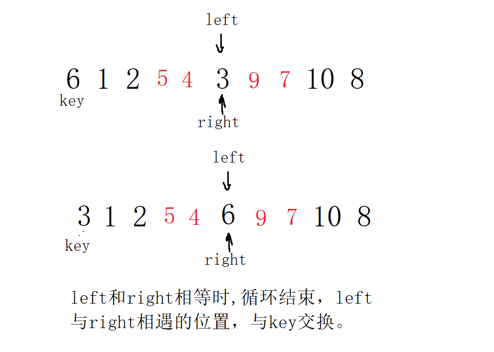
1. Single trip of Hoare version
int Part1Sort(int* a, int left ,int right)
{
int key = left;
while (left < right)
{
while (left <right && a[right] >= a[key])
{
right--;
}
while (left < right && a[left] <= a[key])
{
left++;
}
swap(&a[left], &a[right]);
}
swap(&a[left], &a[key]);
int mid = left;
return mid;
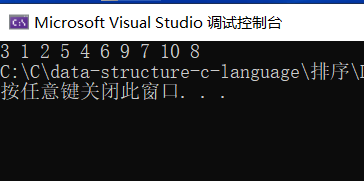
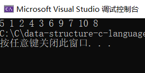
}result:
int main()
{


	int b[] = {6,1,2,7,9,3,4,5,10,8};
	Part1Sort(b,0,(sizeof(b) / sizeof(b[0])-1));

	ArryPrint(b, sizeof(b) / sizeof(b[0]));
	return 0;
}
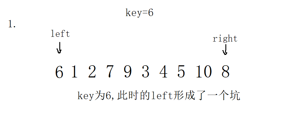
Main process of single trip:
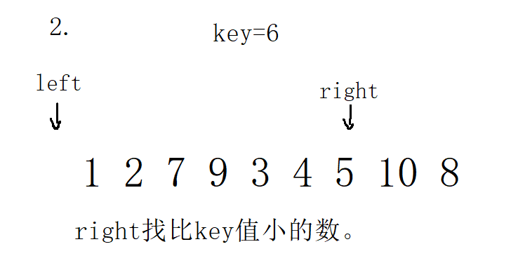
Select the leftmost value as the key, and go first on the right.
Select the value on the far right, and go first on the left
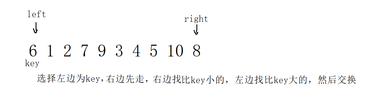
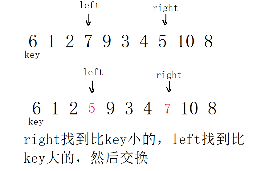
Note that the conditions here should add left < right & & A [right] > = a [key]. When an order is encountered, such as 5 6 7 8 9, and the key is 5, right, go first and find the small, and eventually go directly to the position of 0. If it is not equal to an endless loop, if it is equal to, it will cross the boundary. When it's all 5, without adding the equals sign, it's an endless cycle.
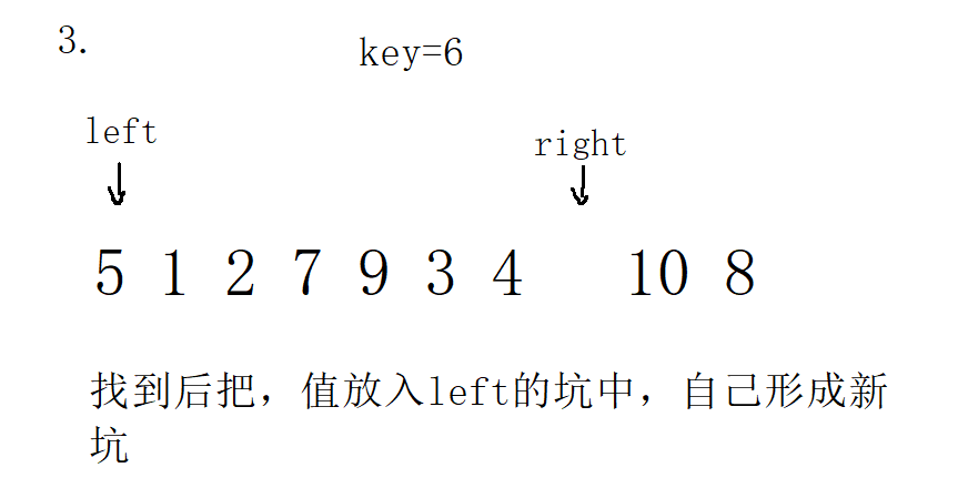
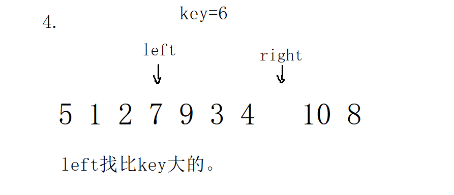
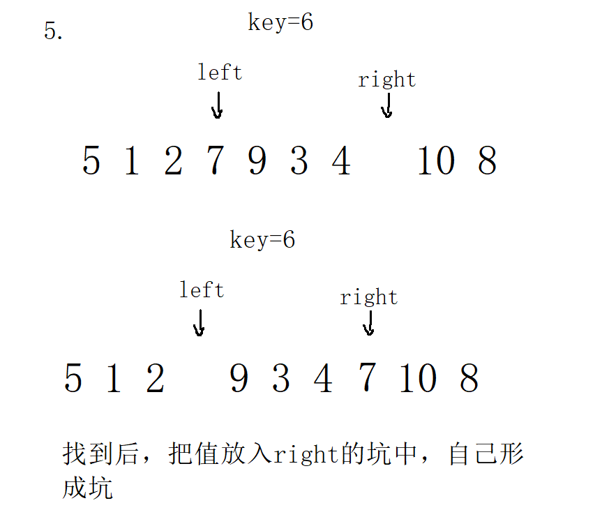
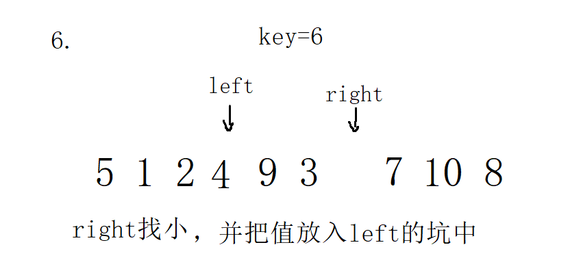
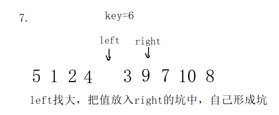
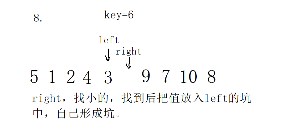
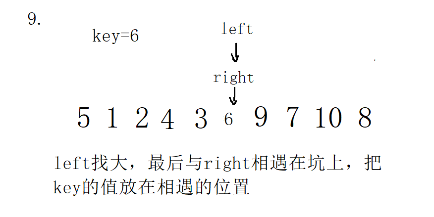
2. Single trip of excavation method
Single trip code of excavation method:
//Excavation method
int Part2Sort(int* a, int left, int right)
{
	int key = a[left];
	while (left <right)
	{
		while (left < right && a[right]>=key)
		{
			right--;
		}
		a[left] = a[right];
		while (left< right && a[left]<=key)
		{
			left++;
		}
		a[right] = a[left];
	}
	a[left] = key;//Will meet in the pit
	return left;//Return the position of the key (middle position)

}
result:
int main()
{

	//int a[] = { 7,2,5,1,4,8,9,6,3,5 };

	int b[] = {6,1,2,7,9,3,4,5,10,8};
	Part2Sort(b,0,(sizeof(b) / sizeof(b[0])-1));

	ArryPrint(b, sizeof(b) / sizeof(b[0]));
	return 0;
}
Process:
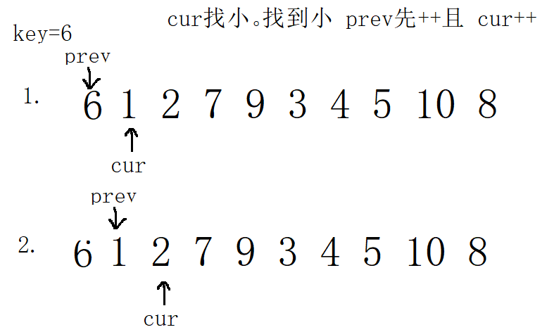
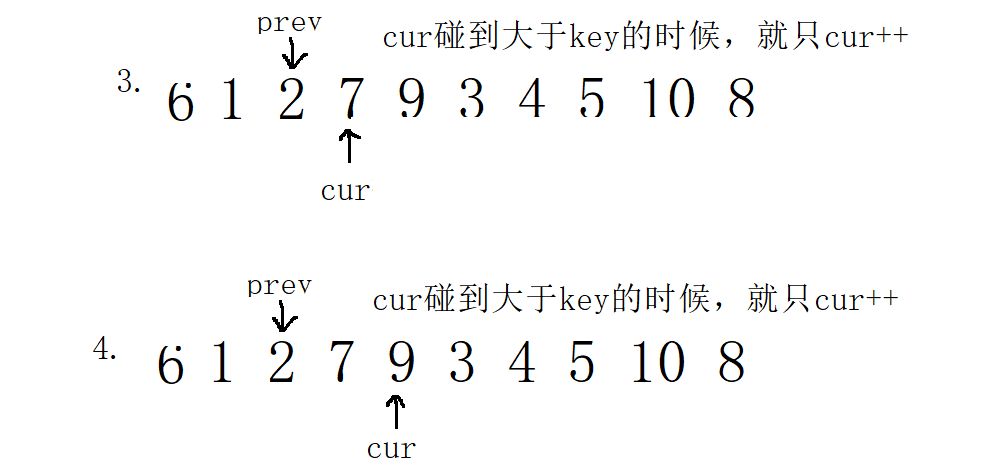
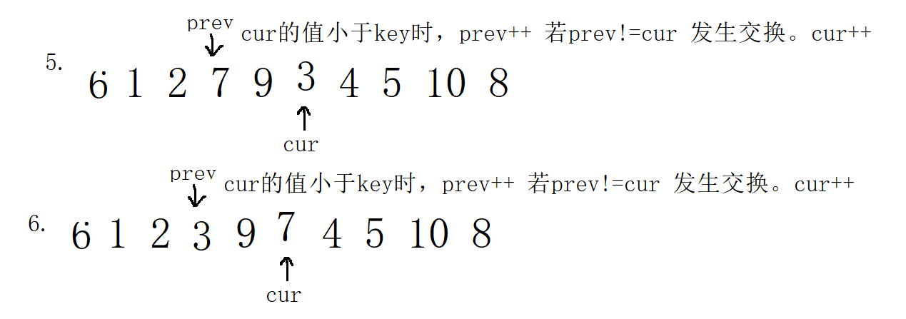
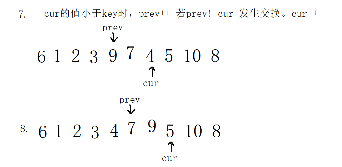
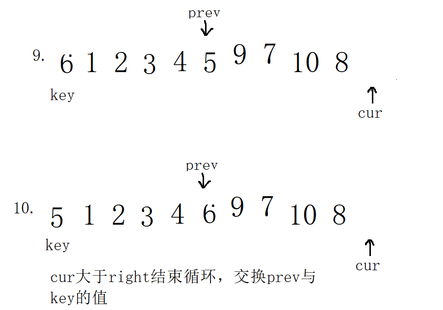
3. Single pass of front and back pointer method
1. In the first case, select key on the left
/Fast and slow pointer method
int Part3Sort(int* a, int left, int right)
{
	//1. Select key on the left, prev=left cur=left+1;

	int prev = left;
	int cur = prev + 1;
	int key= left;
	while (cur <= right)
	{
		if (a[cur] <= a[key] && ++prev !=cur)
		{
			prev++;
			if (prev != cur)
			{
				swap(&a[cur], &a[prev]);
			}
		}
			cur++;

	}
	swap(&a[prev],&a[key]);
	return prev;
}
result:
int main()
{

	//int a[] = { 7,2,5,1,4,8,9,6,3,5 };

	int b[] = {6,1,2,7,9,3,4,5,10,8};
	Part3Sort(b,0,(sizeof(b) / sizeof(b[0])-1));

	ArryPrint(b, sizeof(b) / sizeof(b[0]));
	return 0;
}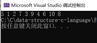
Process:
Complexity analysis of all single trips: the complexity of all single trips is O(N). Compared N times. And each single pass sorting method must return an intermediate value, so that quick sorting can be called directly.
The second step adopts the recursive idea of binary tree. If the left and right sides are orderly, the whole is orderly. It is possible to call any one of the above single pass sorting. The digging method is called here.
Quick sort code:
void QuickSort(int *a ,int left,int right)
{
	if (left >= right)
	{
		return;
	}

	int mid = Part2Sort(a,left,right);
	QuickSort(a, left, mid - 1);
	QuickSort(a, mid + 1, right);
}
Test code:
int main()
{
//int a[] = { 7,2,5,1,4,8,9,6,3,5 };
int b[] = {6,1,2,7,9,3,4,5,10,8};
QuickSort(b,0,(sizeof(b) / sizeof(b[0])-1));
ArryPrint(b, sizeof(b) / sizeof(b[0]));
return 0;
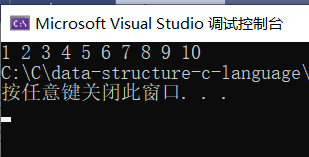
}Results:
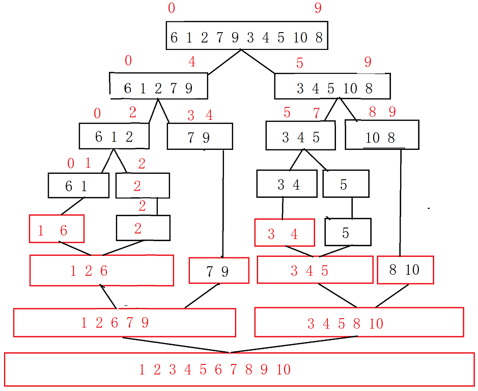
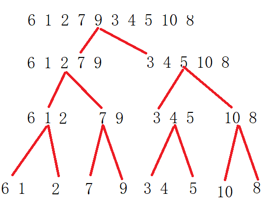
Process: draw more expansion drawings
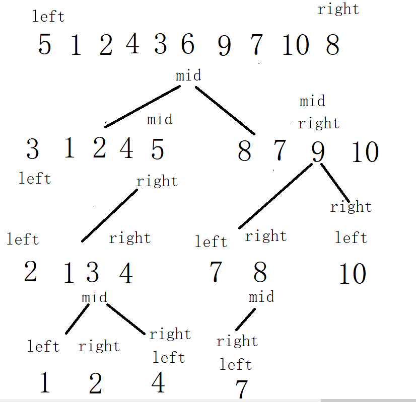
Complexity analysis: each layer is compared N times. How many times are compared in total: height of binary tree times: h=, the total complexity is: O (N*). However, when the array is ordered, such as 1, 2, 3, 4, 5, 6, 7, 8 and 9, the left side is selected as the key every time. Each sorting completes one number. The total number of comparisons is: N-1, N-2, N-3, 1. In this way, it becomes an equal difference sequence, and the complexity becomes O(N^2). In other words, it is very important to select the key for quick sorting. If the selected key is the largest or smallest every time, the complexity is O(N^2). In order to solve this problem, add three numbers to the beginning of the three single pass sorting methods, that is, select the middle value from the three numbers.
The third step is to solve the key selection problem to solve the problem of O(N^2).
Three data access codes: add before each single sequence. Here, take the pit digging method as an example, and others are the same.
int GetMidIndex(int*a ,int left ,int right)
{
	/*int mid =( left+right) / 2;//You can write this
	//int mid = left + (right - left)/2;// Prevent left and right from exceeding half of int and shaping overflow
	int mid = left + ((right - left) >> 1);//Prevent left and right from exceeding half of int and shaping overflow

	if (a[left] < a[mid])
	{
		if (a[mid] < a[right])
			return mid;
		else if (a[left] >a[right])
		{
			return  left;
		}
		else {
			return right;
		}
	}
	//left >mid
	else
	{
		if (a[mid] > a[right])
		{
			return mid;

		}
		else if(a[left]<a[right])
		{
			return left;
		}
		else
		{
			return right;
		}
	}


}
The code uses three data retrieval. Select an intermediate value to exchange with the value of left. When you select key, you still select left. At this time, the value of left has been replaced with the intermediate value.
//Excavation method
int Part2Sort(int* a, int left, int right)
{
    //Triple median
	int mini = GetMidIndex(a, left, right);
	swap(&a[mini], &a[left]);


	int key = a[left];
	while (left <right)
	{
		while (left < right && a[right]>=key)
		{
			right--;
		}
		a[left] = a[right];
		while (left< right && a[left]<=key)
		{
			left++;
		}
		a[right] = a[left];
	}
	a[left] = key;//Will meet in the pit
	return left;//Return the position of the key (middle position)

}
In this way, three data fetching avoids the complexity of O(N^2) caused by the problem that the selected key is either the largest or the smallest in the case of order.
Step 4: inter cell optimization for quick sorting:
According to the characteristics of fast sorting recursion, it is the same as binary tree structure. We assume that the height of the binary tree is 10, the number of nodes in layer 10 is 2 ^ 9 = 512, the number of nodes in layer 9 is 2 ^ 8 = 256, and so on. In other words, the number of nodes in the last layers is the largest. The same is true for the recursion of fast sorting based on binary tree reasoning. There are many recursive calls in the last few layers of recursion, so we can insert sorting when the last few data of the array are left, because we have analyzed that the effect of direct insertion sorting is the best when it is close to order. Therefore, there are the following inter cell code optimization.
void QuickSort(int *a ,int left,int right)
{
	if (left >= right)
	{
		return;
	}
	//Interval optimization of the last few layers of quick sorting,
	if (right - left + 1 < 10)
	{
		InsertSort(a+left,right-left+1);
	}
	else
	{
		int mid = Part2Sort(a, left, right);
		QuickSort(a, left, mid - 1);
		QuickSort(a, mid + 1, right);
	}


}
4.3 quick sort non recursive
Fast platoon also has a dead end: it's all a number, 5, 5, 5, 5, 5, 5 or 2, 3, 2, 3, 2, 3. This is still the worst case, O(N^2), which can't be solved. If there are a lot of data like this, stack overflow will occur if recursion continues. The stack is about 8M on a 32-bit machine, and the heap is 1-2G larger. In order to prevent stack overflow, non recursive write fast sorting is required. The knowledge of stack (stack of data structure) is used.
Quick sort non recursive Code:
//Quick sort non recursive
void QuickSortNonR(int* a, int left, int right)
{
	Stack st;
	StackInit(&st);

	StackPush(&st,left);
	StackPush(&st,right);
	while (!StackEmpty(&st))
	{
		int end=StackTop(&st);//right
		StackPop(&st);
		int begin= StackTop(&st);//left
		StackPop(&st);

		int mid = Part2Sort(a, begin, end);
		//First in right
		if (mid + 1 < end)
		{
			StackPush(&st, mid + 1);
			StackPush(&st, right);
		}
		//Back to the left, first to the left
		if (begin < mid - 1)
		{

			StackPush(&st, left);
			StackPush(&st, mid-1);
		}

	}
	StackDestroy(&st);
}
Test code:
int main()
{
//int a[] = { 7,2,5,1,4,8,9,6,3,5 };
int b[] = {6,1,2,7,9,3,4,5,10,8};
QuickSortNonR(b,0,(sizeof(b) / sizeof(b[0])-1));
ArryPrint(b, sizeof(b) / sizeof(b[0]));
return 0;
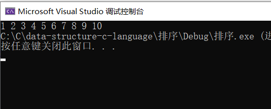
}Results:
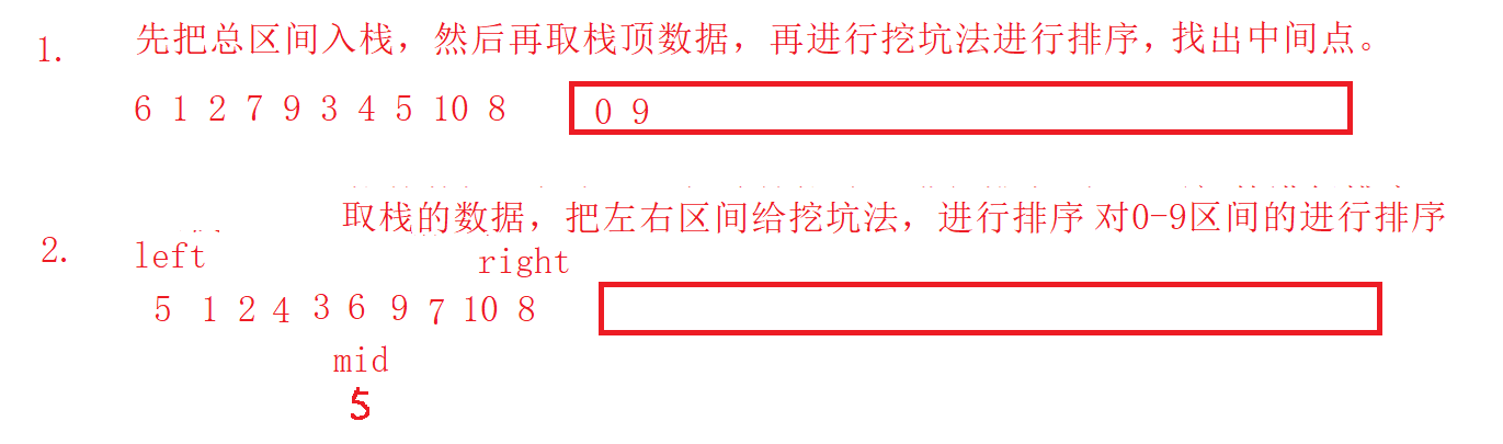
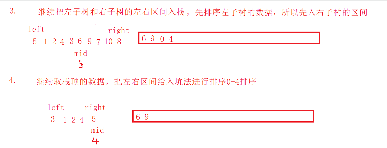
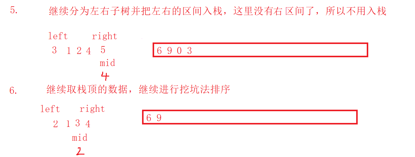
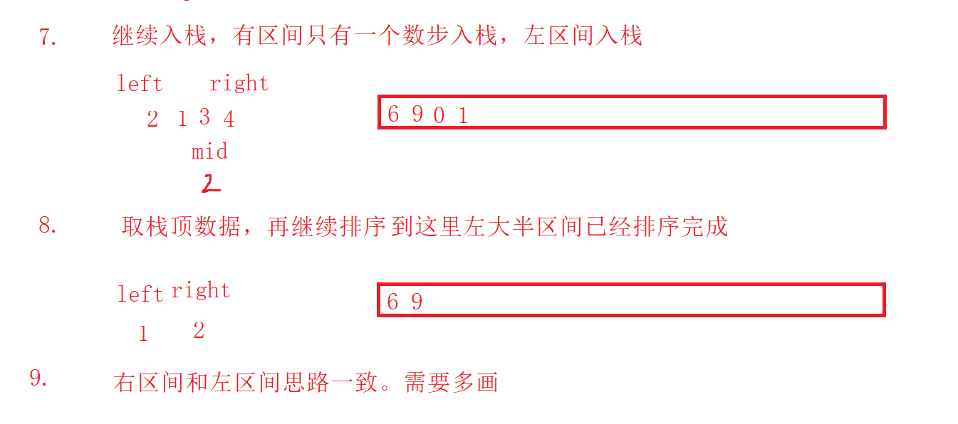
The idea here is consistent with the sequence traversal idea of binary tree. The stack is used to store the left and right recursive intervals. When the left interval is greater than or equal to the right interval, there is no need to sort and stack. We first complete the interval sorting of the left subtree, and then complete the interval sorting of the right subtree. According to the first in and last out of the stack, we need to enter the right interval first.
In the process here, the three numbers are removed. I'm too lazy to calculate, so I can directly analyze:
 5. Merge and sort
5.1 merge sort
int main()
{

	//int a[] = { 7,2,5,1,4,8,9,6,3,5 };

	int b[] = {6,1,2,7,9,3,4,5,10,8};
	MergeSort(b,(sizeof(b) / sizeof(b[0])));

	ArryPrint(b, sizeof(b) / sizeof(b[0]));
	return 0;
}
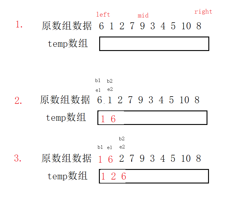
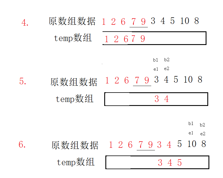
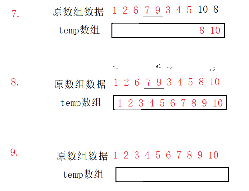
Merge sort code implementation:
//Merged recursive function
void _MergeSort(int* a, int left, int right, int* temp)
{
	if (left >= right)
		return;

	int mid = (left + right)/2 ;
	_MergeSort(a,left,mid,temp);
	_MergeSort(a,mid+1,right,temp);

	int begin1 = left, end1 = mid ;
	int begin2 = mid+1, end2 = right;
	int i = left;

	while (begin1 <=end1 && begin2 <=end2)
	{
		if (a[begin1] < a[begin2])
		{
			temp[i++] = a[begin1++];
		}
		else
		{
			temp[i++] = a[begin2++];
		}
	}
	//Put one of the remaining ordered sequences into the temp array
	while (begin1 <= end1)
	{
		temp[i++] = a[begin1++];
	}
	while (begin2 <= end2)
	{
		temp[i++] = a[begin2++];
	}
	//Put the temp ordered data back into the a array
	for (int j = left; j <= right; j++)
	{
		a[j] = temp[j];
	}
}


//Merge sort
void MergeSort(int* a, int n)
{
	int* temp = (int*)malloc(n*sizeof(int));
	if (temp == NULL)
	{
		printf("Request dynamic memory error\n");
		exit(-1);
	}
	_MergeSort(a,0,n-1,temp);
    free(temp);
	temp = NULL;
}
Results:
Process:
Complexity analysis: each layer has O(N). A total of logN times have been compared. The complexity is O(N*logN).
5.2 merge sort non recursive
Recursive code implementation:
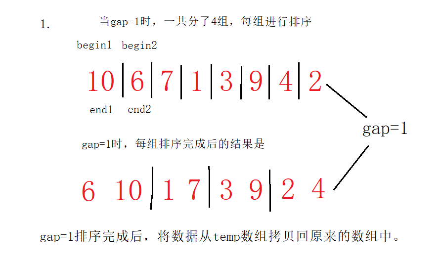
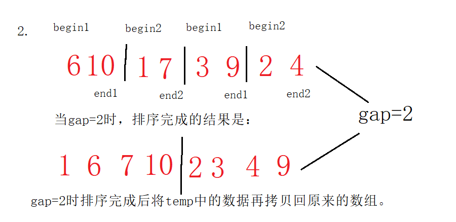
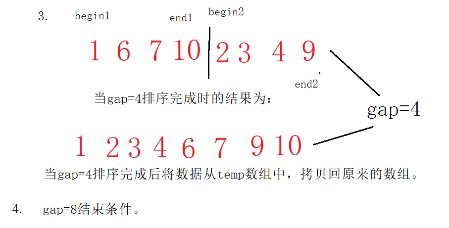
In this case, after merging in the temp array every time, I copy back to the original array. For example, when gap=1, all data are merged in the temp array. After merging, I copy the original array, and then continue gap=2;
//Return is not recursive
void MergeSortNonR(int*a ,int n)
{
	int* temp = (int*)malloc(n*sizeof(int));
	if (temp == NULL)
	{
		printf("Application failed\n");
		exit(-1);
	}
	int gap = 1;
	while (gap<n)
	{
		for (int i = 0; i < n; i+=gap*2)
		{
			int begin1 = i, end1 = i + gap - 1;
			int begin2 = i + gap, end2 = i + 2 * gap - 1;
			int j = i;

			//Solve three cases of interval
			if (end1 >= n)
			{
				end1 = n - 1;
			}
			if (begin2 >=n)
			{
				begin2 = n;//Interval does not exist
				end2 = n - 1;
			}
			if (end2 >= n)
			{
				end2 = n - 1;
			}


			while (begin1 <= end1 && begin2 <= end2)
			{
				if (a[begin1] < a[begin2])
				{
					temp[j++] = a[begin1++];

				}
				else
				{
					temp[j++] = a[begin2++];
				}
			}
			while (begin1 <= end1)
			{
				temp[j++] = a[begin1++];
			}
			while (begin2 <= end2)
			{
				temp[j++] = a[begin2++];
			}
		}
		for (int j = 0; j < n; j++)
		{
			a[j] = temp[j];
		}
		gap *= 2;

	}

	free(temp);
	temp = NULL;

}
Test code:
int main()
{

	//int a[] = { 7,2,5,1,4,8,9,6,3,5 };

	int b[] = {10,6,7,1,3,9,4,2};
	MergeSortNonR(b,sizeof(b) / sizeof(int));

	ArryPrint(b, sizeof(b) / sizeof(b[0]));
	return 0;
}
Results: the result is that the 8 numbers do not cross the boundary. Analyze the 8 numbers first.
Process: there is no cross-border situation in this process, which can be divided into two situations: one is not cross-border situation, and the other is to analyze cross-border situation.
1. Process of non crossing:
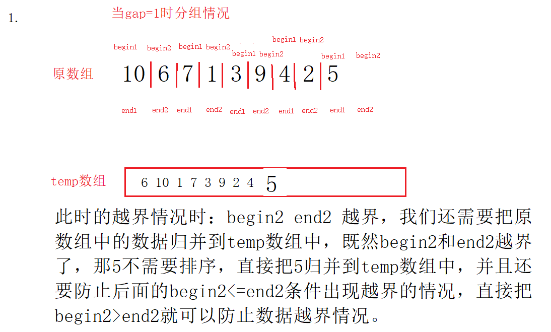
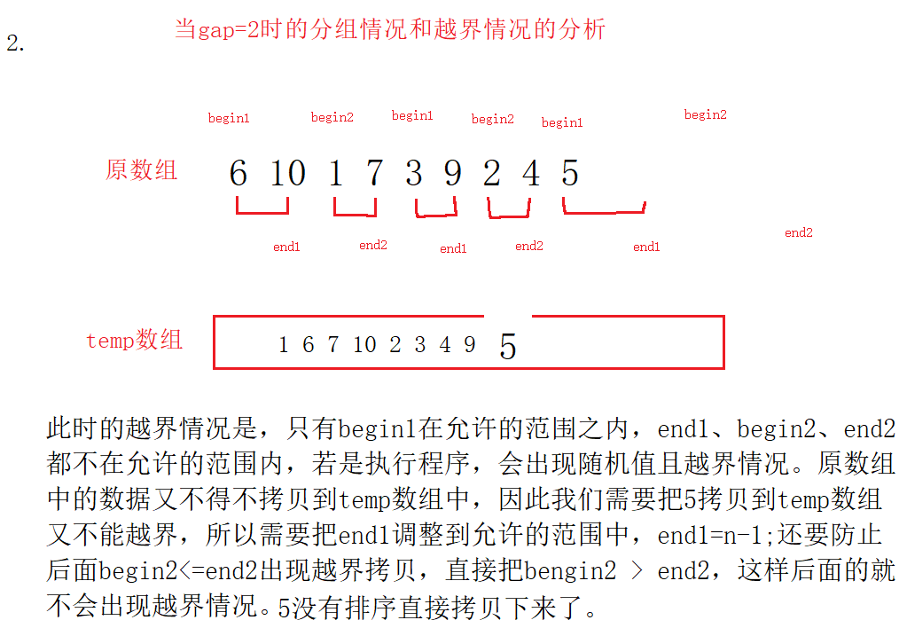
 2. Out of bounds: a data element is added to the original array element 5.
int main()
{
//int a[] = { 7,2,5,1,4,8,9,6,3,5 };
int b[] = {10,6,7,1,3,9,4,2,5};
MergeSortNonR(b,sizeof(b) / sizeof(int));
ArryPrint(b, sizeof(b) / sizeof(b[0]));
return 0;
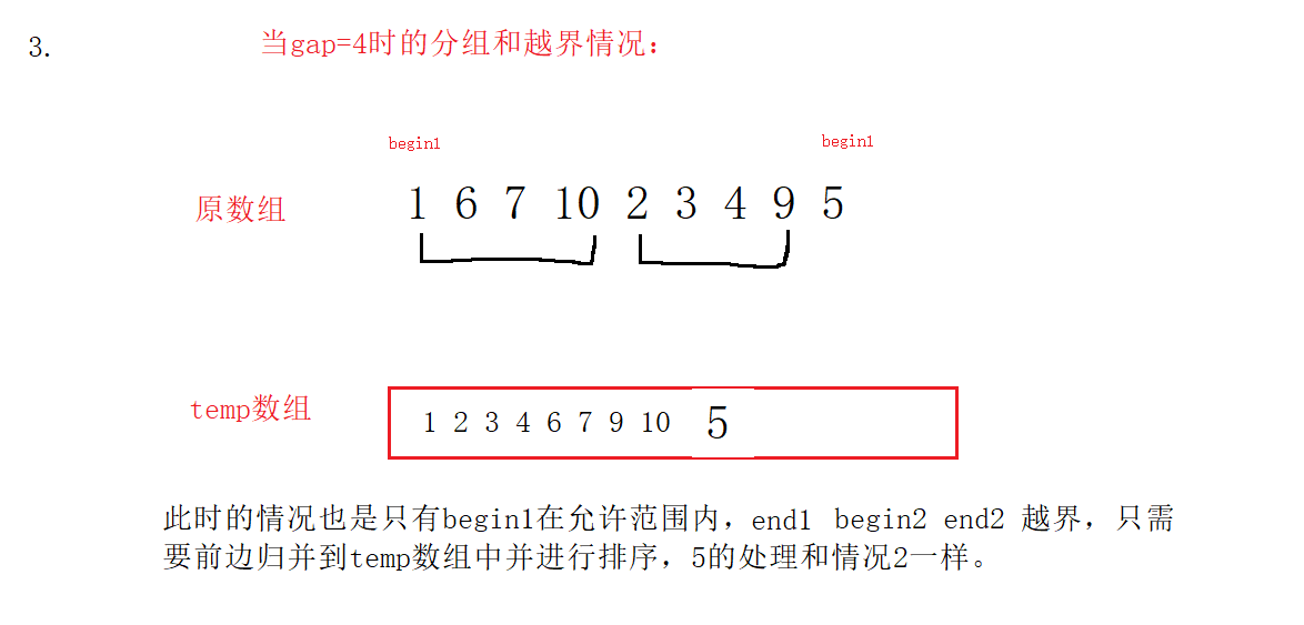
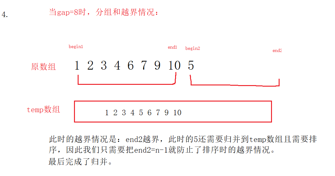
}The cross-border situations are mainly divided into the following situations: 1 Begin2 end2 out of bounds 2 En1 begin2 end2 out of bounds 3 End2 out of bounds
3. Another way to solve the cross-border situation: modify the writing method of the code. Like recursion, merge and copy back once at a time.
void MergeSortNonR1(int* a, int n)
{
	int* temp = (int*)malloc(n * sizeof(int));
	if (temp == NULL)
	{
		printf("Application failed\n");
		exit(-1);
	}
	int gap = 1;
	while (gap < n)
	{
		for (int i = 0; i < n; i += gap * 2)
		{
			int begin1 = i, end1 = i + gap - 1;
			int begin2 = i + gap, end2 = i + 2 * gap - 1;
			int j = i;

            //Cross boundary correction

			if (end1 >= n || begin2>=n)
			{
				break;
			}
			if (end2 >= n)
			{
				end2 = n - 1;
			}


			while (begin1 <= end1 && begin2 <= end2)
			{
				if (a[begin1] < a[begin2])
				{
					temp[j++] = a[begin1++];

				}
				else
				{
					temp[j++] = a[begin2++];
				}
			}
			while (begin1 <= end1)
			{
				temp[j++] = a[begin1++];
			}
			while (begin2 <= end2)
			{
				temp[j++] = a[begin2++];
			}

            //Modified part

			for (int j = i; j <= end2; j++)
			{
				a[j] = temp[j];
			}
		}

		gap *= 2;

	}

	free(temp);
	temp = NULL;

}
Complexity analysis of merging sorting: it can be understood as a binary tree, with the height of h=logN, each sorting O(N), the total complexity is O(N)*logN, and the spatial complexity is O(N).
6. Non comparative sorting
6.1 counting and sorting (selection and mastery)
1. Integer array suitable for comparison set
2. A large range or floating-point numbers are not suitable for counting and sorting.
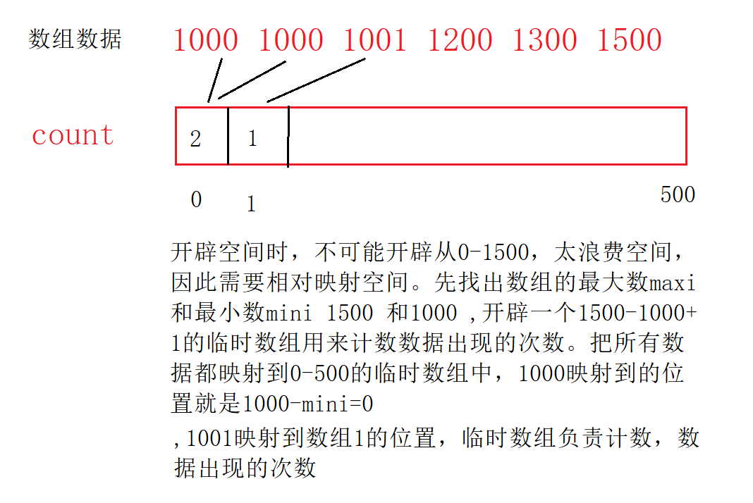
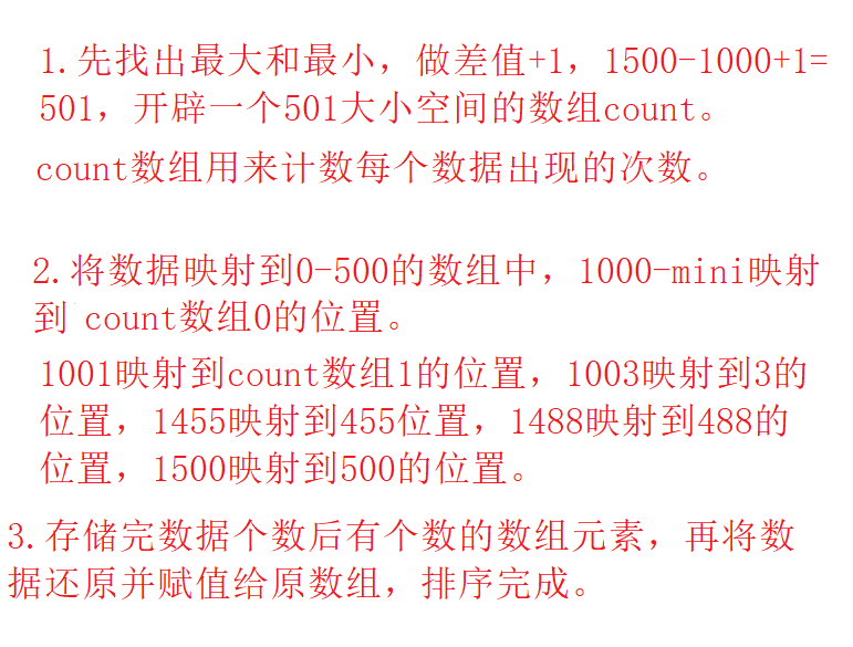
Relative mapping of location:
Count sort code:
void CountSort(int* a, int n)
{
	//Find the maximum and minimum first
	int maxi = a[0];
	int mini = a[0];
	for (int i = 1; i < n; i++)
	{
		if (a[i] > maxi)
		{
			maxi = a[i];
		}
		if (a[i]<mini)
		{
			mini = a[i];

		}
	}

    //Specifies the size of the temporary array
	int range =maxi - mini + 1;
	int* count = (int*)malloc(range*sizeof(int));

	if (count == NULL)
	{
		printf("Application failed\n");
		exit(-1);
	}

	memset(count,0,sizeof(int)*range);//Clear
    //The array data is mapped to the corresponding position and counted
	for (int j=0;j<n;j++)
	{
		count[a[j] - mini]++;//Count, relative mapping
	}
    //Return the data to the original array.
	int j = 0;
	for (int i=0;i<range;i++ )
	{

		while (count[i]--)
		{
			a[j++] =i + mini;
		}
	}

	free(count);
	count = NULL;
}
int main()
{


	int b[] = {1000,1500,1001,1003,1488,1455};
	CountSort(b,sizeof(b) / sizeof(int));

	ArryPrint(b, sizeof(b) / sizeof(b[0]));
	return 0;
}
result:
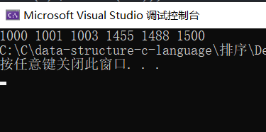
Process:
Count sorting complexity analysis: O(MAX(N,range)). It is necessary to traverse the original array O(N) and assign the number in the count array back to the original array through calculation. It is also necessary to traverse the count array O(range). Therefore, the complexity is O(MAX(N,range)).
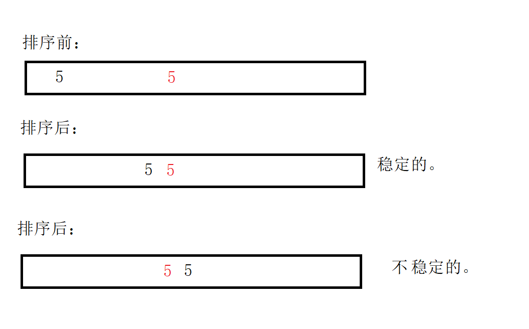
7. Ranking stability summary
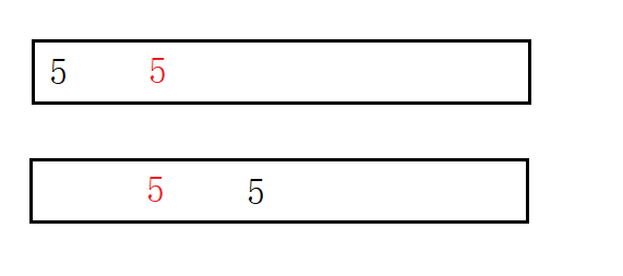
Stability: whether the relative position of the same value in the array changes after sorting. May become unstable. If you can guarantee invariance, you are stable.
Meaning: for the same score, there is only one place for the first prize. How to rank? Therefore, according to the order of submission, ensure that the ranking is stable and will not be disordered. Whoever hands in the paper first will win the first prize.
For example:
Insertion sorting: 1 2 3 4 5 6 can ensure stability. So the insertion sort is stable.
Hill sorting: there is no guarantee that instability will occur when the same data is divided into different groups. So hill is unstable.
Select Sorting: 5 1 2 3 5 0 6, find one number at a time, find the small one first, and the first number 5 will be changed to the position of 0. Therefore, it is unstable.
Heap sort:
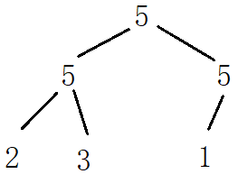 In this case, if the row is in ascending order, instability may occur, so the heap row is unstable.
Bubble sorting: it can ensure stability. So it's stable.
Quick sort: assume that the key is 5, and finally change to the middle position. Therefore, it is unstable.
Merge sort: it can be stable. When merging, you can merge the left 2 first, and merge the right one.