Introduction to Spark SQL
Spark SQL is one of the most complex components in spark technology. It provides the function of operating structured data in Spark Program, that is, SQL query. Specifically, spark SQL has the following three important features:
1.Spark SQL supports reading of multiple structured data formats, such as JSON,Parquet or Hive tables.
2.Spark SQL supports reading data from a variety of external data sources. In addition to local data, HDFS and S3, it can also connect to external relational database systems through standard database connectors such as JDBC.
3. The last point is to be able to freely perform SQL operations in Spark programs and achieve a high degree of integration with various programming languages Python/Java/Scala.
In order to realize these important functions, Spark SQL introduces a special RDD called DataFrame, which is also called schemardd (before spark 1.3.0).
Let's take a look at DataFrame first.
DataFrame theory
DataFrame is a distributed data set based on RDD. Theoretically, it is very close to a data table in relational database or the data abstract Data Frame in Python pandas.
However, compared with the DataFrame in Python or R, the DataFrame in Spark SQL is more optimized internally during execution. First, like ordinary RDD, the DataFrame also abides by the inert mechanism, that is, the real calculation is only when action (such as displaying results or saving output) is triggered. It is precisely because of this mechanism that Spark SQL DataFrame based operations can be optimized automatically.
The core optimizer behind Spark SQL is called Catalyst Optimizer. Let me introduce Catalyst workflow in detail based on the following figure.
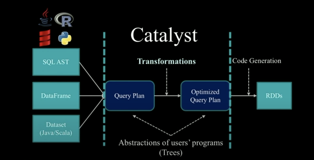
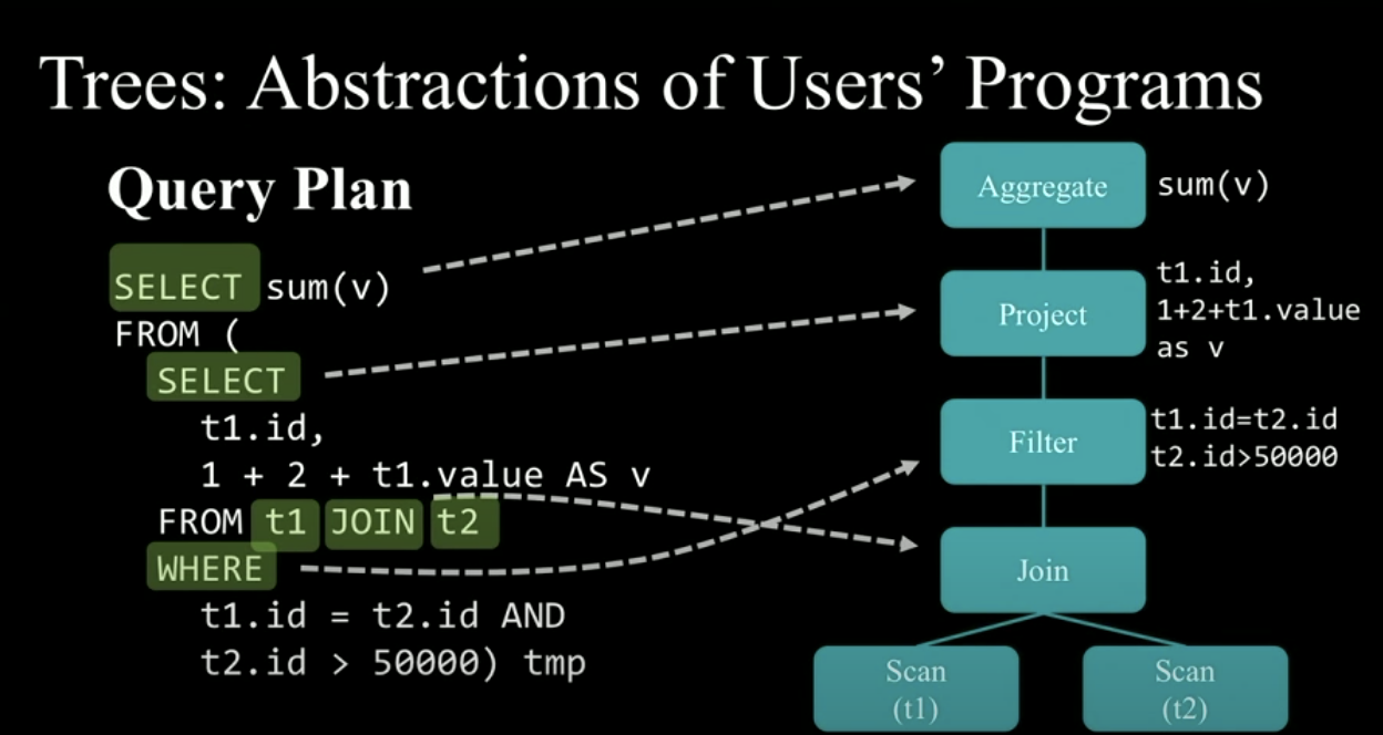
First, the selected DataFrame/Dataset and the corresponding SQL statement will be received by Catalyst as input and generate an unprocessed Query Plan. Each Plan uses a tree as an abstract set of user programs, and its nodes are used to describe a series of operation processes from the input dataset to the output query results. Each node corresponds to a step. The following is a simple example example.
Then, through a series of transformations between trees, the Optimized Query Plan is obtained from the initial Query Plan to generate RDD DAG for subsequent execution. The internal structure of the transformation operation is as follows.
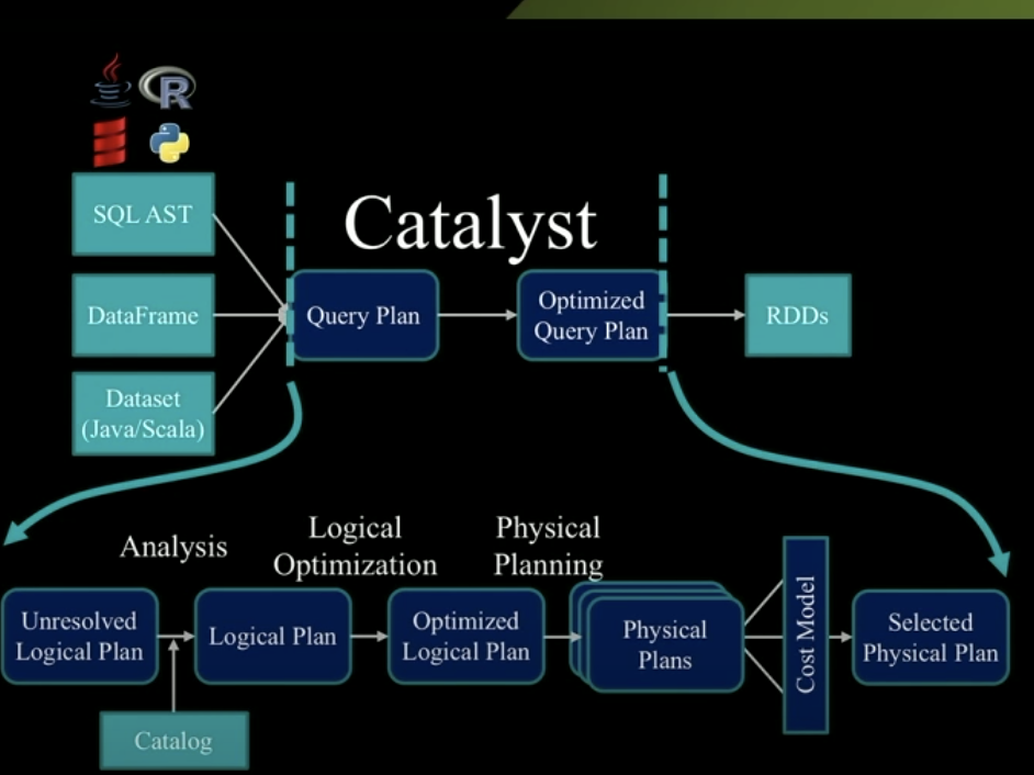
The whole optimization process is concentrated in the Transformation part, so how to carry out the Transformation? Before summarizing the complete Transformation process, let's briefly introduce the two concepts involved in the Transformation process.
1.Logical Plan: it defines the related calculation operations involved in the user's query statement, but does not include the specific calculation process.
2.Physical Plan: it specifically describes the operation flow of the input data set, so it is executable.
Next, let's take a look at how Transformation is transformed. In the whole Transformation process, there are two different types of transformations, the mutual Transformation between similar trees and the mutual Transformation between different kinds of trees.
Let's first look at the first transformation, that is, the transformation between similar trees, such as the transformation from Logical Plan to Optimized Logical Plan. In Spark, each single transformation is defined by a rule, and each rule corresponds to a function, which is called transform. Generally, we are used to combining multiple single rule s to form a complete rule The following is an example of a part of the conversion process.
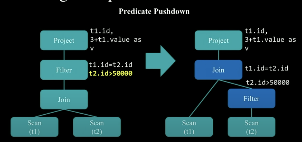
The above conversion process involves a very typical optimization step, called Predicate Pushdown. That is, press the filter predicate to the specified data source, the t2 table in the figure above. First filter the t2 table, and then join the filtered results. This avoids unnecessary data joins and effectively increases the efficiency of joins.
This combination of multiple rules is also called Rule Executor, that is, a Rule Executor converts a tree into another tree of the same category by using multiple rules.
Next, let's take a look at the second transformation - the transformation between different category trees, from Logical Plan to Physical Plan. A series of policies are used. Each policy corresponds to the transformation process from a node of Logical Plan to a corresponding node of Physical Plan. The operation of each policy will trigger the start of subsequent policies.
OK, finally, let's completely comb through the optimization process of Catalyst.
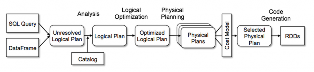
1.Analysis: use Rule Executor to convert Unresolved Logical Plan to Resolved Logical Plan.
2.Logical Optimization: use another Rule Executor to convert the Resolved Logical Plan to the Optimized Logical Plan.
3.Physical Planning: this part is divided into two stages. Stage 1: convert the Optimized Logical Plan into Physical Plan through Strategies. Stage 2: adjust it through Rule Executor for final execution.
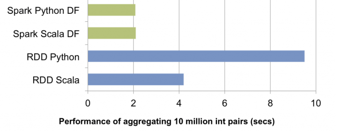
The above is a brief introduction to Catalyst Optimizer. Another point worth mentioning is that for Python users, that is, PySpark, another advantage of Catalyst Optimizer is that it can significantly improve the use efficiency of PySpark. In other words, compared with using RDD in PySpark, the query efficiency of using DataFrame will be greatly improved. The reason is very simple, because For Catalyst Optimizer, no matter what language the initial code is written in, the final optimizer will uniformly generate JVM binary code for execution. Therefore, when using DataFrame, the execution speed is not affected by the programming language. However, if it is RDD, the execution speed of Python will be much slower than that of Java or Scala, which also performs RDD operations. The main reason is It is the overhead of Python and JVM in the process of communication. We can take a look at the following figure to intuitively feel it.
DataFrame practices
Having finished the important optimizer behind Spark SQL, we now officially enter the introduction to the use of DataFrame. Here we take PySpark as an example.
First, we need to create a SparkSession. Before Spark 2,0, we will use SQLContext. Meanwhile, Spark has many other contexts, such as HiveContext, StreamingContext, and SparkContext, which are now unified into SparkSession.
from pyspark import SparkConf,SparkContext
from pyspark.sql import SparkSession

conf=SparkConf().setMaster('local').setAppName('sparksql')
sc=SparkContext(conf=conf)

spark=SparkSession.builder.appName('sparksql').master('local').getOrCreate()
We have a JSON file std_info.json that briefly describes student information. We use SparkSession to read it in.
[{"id": "123", "name": "Katie", "age": 19, "eyeColor": "brown"},
 {"id": "234", "name": "Michael", "age": 22, "eyeColor": "green"},
 {"id": "345", "name": "Simone", "age": 23, "eyeColor": "blue"}]
df=spark.read.json('std_info.json') # Generate DataFrame
df.show()
# Return results
+---+--------+---+-------+
|age|eyeColor| id|   name|
+---+--------+---+-------+
| 19|   brown|123|  Katie|
| 22|   green|234|Michael|
| 23|    blue|345| Simone|
+---+--------+---+-------+
In addition to using the. show() method to view the data contained in the DataFrame, we can also use. collect() and. Take (n). N represents the number of rows we want to get, and the returned row object will be stored in the list and returned.
# We can also view column information
df.printSchema()
# Return results
root
 |-- age: long (nullable = true)
 |-- eyeColor: string (nullable = true)
 |-- id: string (nullable = true)
 |-- name: string (nullable = true)
Data query using DataFrame API
Next, we use the DataFrame API to query the data.
1. We can use the. count() method to check the number of rows in the DataFrame.
df.count()

# Return results
3
2. We can combine. select() and. filter() for conditional filtering.
# Query students aged 22
df.select('id','age').filter('age=22').show()
# or
df.select(df.id,df.age).filter(df.age==22).show()
# Return results
+---+---+
| id|age|
+---+---+
|234| 22|
+---+---+
# Query students whose eye color begins with the letter b
df.select('name','eyeColor').filter('eyeColor like "b%"').show()
# Return results
+------+--------+
|  name|eyeColor|
+------+--------+
| Katie|   brown|
|Simone|    blue|
+------+--------+
Data query using SQL
We use SQL to perform the same query task as above, using spark.sql(). It should be noted that when we need to perform SQL query on the DataFrame, we need to register the DataFrame as a Table or View.
df.createOrReplaceTempView("df")
1. Query the number of rows.
spark.sql(" select count(1) from df" ).show()
# Return results
+--------+
|count(1)|
+--------+
|       3|
+--------+
2. Query students aged 22
spark.sql('select id,age from df where age=22').show()
# Return results
+---+---+
| id|age|
+---+---+
|234| 22|
+---+---+
3. Query students whose eye color begins with the letter b
spark.sql('select name,eyeColor from df where eyeColor like "b%"').show()
# Return results
+------+--------+
|  name|eyeColor|
+------+--------+
| Katie|   brown|
|Simone|    blue|
+------+--------+
How to convert RDD to DataFrame
RDD - > dataframe is a data structured process. We need to customize the schema. Let's look at the following example.
# import types is used for schema definition
from pyspark.sql.types import *

# Creating an RDD is consistent with the information contained in the above example
rdd=sc.parallelize([
(123,'Katie',19,'brown'),
(234,'Michael',22,'green'),
(345,'Simone',23,'blue')
])

# Define schema
schema = StructType([
   StructField("id", LongType(), True),
   StructField("name", StringType(), True),
   StructField("age", LongType(), True),
   StructField("eyeColor", StringType(), True)
   ])

#Create DataFrame
rdd2df = spark.createDataFrame(rdd, schema)
rdd2df.show()
# Return results
+---+-------+---+--------+
| id|   name|age|eyeColor|
+---+-------+---+--------+
|123|  Katie| 19|   brown|
|234|Michael| 22|   green|
|345| Simone| 23|    blue|
+---+-------+---+--------+
summary
OK, so far, the basic theoretical background and basic DataFrame operation of Spark SQL have been introduced. I hope it will be helpful to you!
reference resources
1.Learning PySpark. Tomasz Drabas, Denny Lee
2.Introducing DataFrames in Apache Spark for Large Scale Data Science