Hello, I'm little F.

Today I'd like to introduce you to a wonderful spatial (Geographic) data visualization artifact: Pydeck.

Pydeck library through deck GL carries out spatial visual rendering of data, and has strong support for 3D visualization.

Working with documents:

https://pydeck.gl/index.html

GitHub:

https://github.com/visgl/deck.gl/tree/master/bindings/pydeck

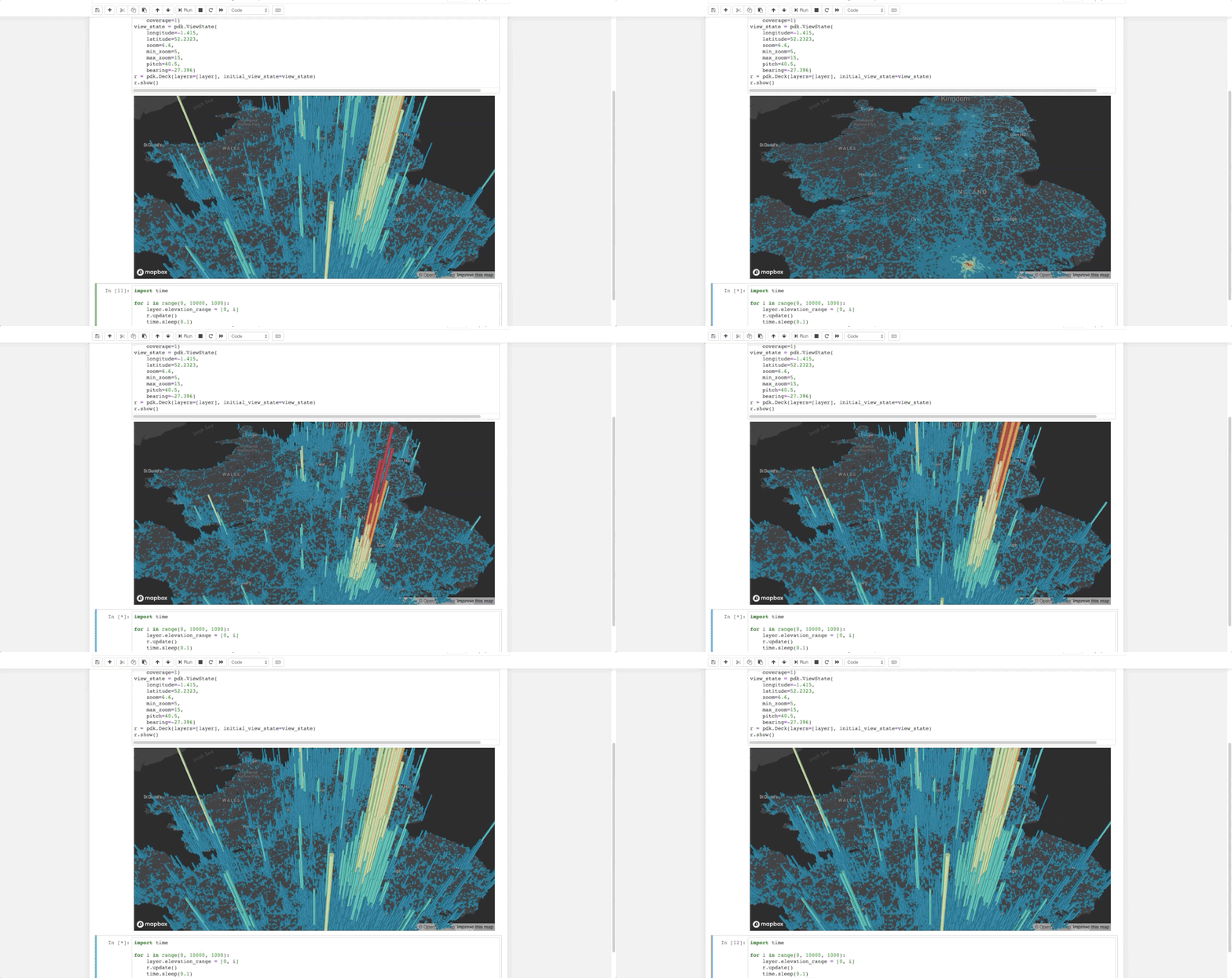
Install with the following command.

# install
pip install pydeck -i https://mirror.baidu.com/pypi/simple

It can be run on jupyter notebook and IDE, and relevant plug-ins need to be installed on jupyter.

# Enable Pydeck
jupyter nbextension install --sys-prefix --symlink --overwrite --py pydeck
jupyter nbextension enable --sys-prefix --py pydeck

Next, let's introduce relevant visualization cases.

The data and codes used have been uploaded and can be obtained at the end of the text~

① Arc diagram

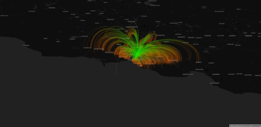
The commute of workers after work starts from downtown San Francisco (green) and ends at the destination (red).

The data were collected by the U.S. Census Bureau.

Address:

https://lehd.ces.census.gov/data/

The code is as follows.

import pydeck as pdk
import pandas as pd

DATA_URL = "https://raw.githubusercontent.com/ajduberstein/sf_public_data/master/bay_area_commute_routes.csv"
# A bounding box for downtown San Francisco, to help filter this commuter data
DOWNTOWN_BOUNDING_BOX = [
    -122.43135291617365,
    37.766492914983864,
    -122.38706428091974,
    37.80583561830737,
]


def in_bounding_box(point):
    """Determine whether a point is in our downtown bounding box"""
    lng, lat = point
    in_lng_bounds = DOWNTOWN_BOUNDING_BOX[0] <= lng <= DOWNTOWN_BOUNDING_BOX[2]
    in_lat_bounds = DOWNTOWN_BOUNDING_BOX[1] <= lat <= DOWNTOWN_BOUNDING_BOX[3]
    return in_lng_bounds and in_lat_bounds


df = pd.read_csv(DATA_URL)
# Filter to bounding box
df = df[df[["lng_w", "lat_w"]].apply(lambda row: in_bounding_box(row), axis=1)]

GREEN_RGB = [0, 255, 0, 40]
RED_RGB = [240, 100, 0, 40]

# Specify a deck.gl ArcLayer
arc_layer = pdk.Layer(
    "ArcLayer",
    data=df,
    get_width="S000 * 2",
    get_source_position=["lng_h", "lat_h"],
    get_target_position=["lng_w", "lat_w"],
    get_tilt=15,
    get_source_color=RED_RGB,
    get_target_color=GREEN_RGB,
    pickable=True,
    auto_highlight=True,
)

view_state = pdk.ViewState(latitude=37.7576171, longitude=-122.5776844, bearing=45, pitch=50, zoom=8,)


TOOLTIP_TEXT = {"html": "{S000} jobs <br /> Home of commuter in red; work location in green"}
r = pdk.Deck(arc_layer, initial_view_state=view_state, tooltip=TOOLTIP_TEXT)
r.to_html("arc_layer.html")

② 3D histogram

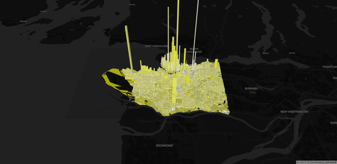
For the house price situation in Vancouver, Canada, the input data is in GeoJSON format.

The code is as follows.

import pydeck as pdk

DATA_URL = "https://raw.githubusercontent.com/visgl/deck.gl-data/master/examples/geojson/vancouver-blocks.json"
LAND_COVER = [[[-123.0, 49.196], [-123.0, 49.324], [-123.306, 49.324], [-123.306, 49.196]]]

INITIAL_VIEW_STATE = pdk.ViewState(latitude=49.254, longitude=-123.13, zoom=11, max_zoom=16, pitch=45, bearing=0)

polygon = pdk.Layer(
    "PolygonLayer",
    LAND_COVER,
    stroked=False,
    # processes the data as a flat longitude-latitude pair
    get_polygon="-",
    get_fill_color=[0, 0, 0, 20],
)

geojson = pdk.Layer(
    "GeoJsonLayer",
    DATA_URL,
    opacity=0.8,
    stroked=False,
    filled=True,
    extruded=True,
    wireframe=True,
    get_elevation="properties.valuePerSqm / 20",
    get_fill_color="[255, 255, properties.growth * 255]",
    get_line_color=[255, 255, 255],
)

r = pdk.Deck(layers=[polygon, geojson], initial_view_state=INITIAL_VIEW_STATE)

r.to_html("geojson_layer.html")

③ Icon diagram

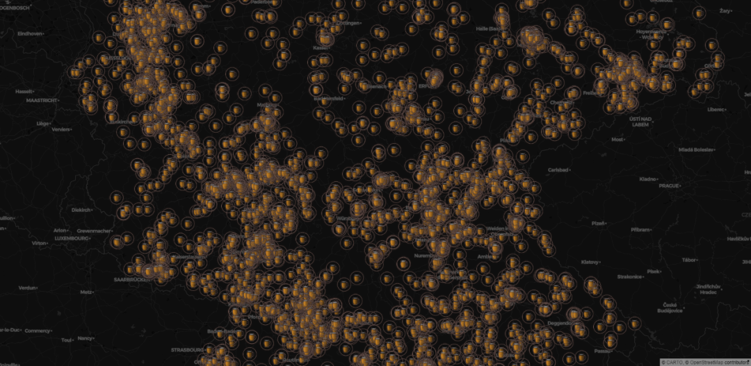
Location and distribution of beer gardens in Germany.

The code is as follows.

import pydeck as pdk
import pandas as pd


# Data from OpenStreetMap, accessed via osmpy
DATA_URL = "https://raw.githubusercontent.com/ajduberstein/geo_datasets/master/biergartens.json"
ICON_URL = "https://upload.wikimedia.org/wikipedia/commons/c/c4/Projet_bi%C3%A8re_logo_v2.png"

icon_data = {
    # Icon from Wikimedia, used the Creative Commons Attribution-Share Alike 3.0
    # Unported, 2.5 Generic, 2.0 Generic and 1.0 Generic licenses
    "url": ICON_URL,
    "width": 242,
    "height": 242,
    "anchorY": 242,
}

data = pd.read_json(DATA_URL)
data["icon_data"] = None
for i in data.index:
    data["icon_data"][i] = icon_data

view_state = pdk.data_utils.compute_view(data[["lon", "lat"]], 0.1)

icon_layer = pdk.Layer(
    type="IconLayer",
    data=data,
    get_icon="icon_data",
    get_size=4,
    size_scale=15,
    get_position=["lon", "lat"],
    pickable=True,
)

r = pdk.Deck(layers=[icon_layer], initial_view_state=view_state, tooltip={"text": "{tags}"})
r.to_html("icon_layer.html")

④ Flow diagram

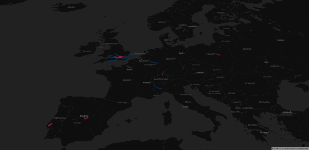
Flight route map from Heathrow airport to all parts of Europe.

The code is as follows.

import pydeck as pdk

DATA_URL = {
    "AIRPORTS": "https://raw.githubusercontent.com/visgl/deck.gl-data/master/examples/line/airports.json",
    "FLIGHT_PATHS": "https://raw.githubusercontent.com/visgl/deck.gl-data/master/examples/line/heathrow-flights.json",  # noqa
}

INITIAL_VIEW_STATE = pdk.ViewState(latitude=47.65, longitude=7, zoom=4.5, max_zoom=16, pitch=50, bearing=0)

# RGBA value generated in Javascript by deck.gl's Javascript expression parser
GET_COLOR_JS = [
    "255 * (1 - (start[2] / 10000) * 2)",
    "128 * (start[2] / 10000)",
    "255 * (start[2] / 10000)",
    "255 * (1 - (start[2] / 10000))",
]

scatterplot = pdk.Layer(
    "ScatterplotLayer",
    DATA_URL["AIRPORTS"],
    radius_scale=20,
    get_position="coordinates",
    get_fill_color=[255, 140, 0],
    get_radius=60,
    pickable=True,
)

line_layer = pdk.Layer(
    "LineLayer",
    DATA_URL["FLIGHT_PATHS"],
    get_source_position="start",
    get_target_position="end",
    get_color=GET_COLOR_JS,
    get_width=10,
    highlight_color=[255, 255, 0],
    picking_radius=10,
    auto_highlight=True,
    pickable=True,
)

layers = [scatterplot, line_layer]

r = pdk.Deck(layers=layers, initial_view_state=INITIAL_VIEW_STATE)
r.to_html("line_layer.html")

⑤ Path map

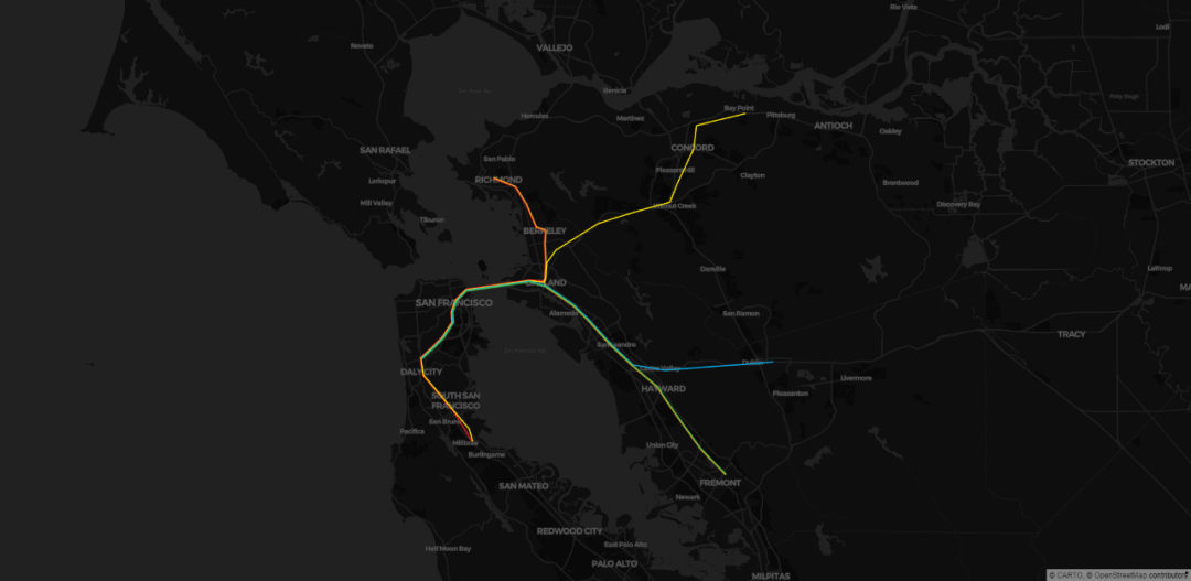
Bay area rapid transit route map.

The code is as follows.

import pandas as pd
import pydeck as pdk

DATA_URL = "https://raw.githubusercontent.com/visgl/deck.gl-data/master/website/bart-lines.json"
df = pd.read_json(DATA_URL)


def hex_to_rgb(h):
    h = h.lstrip("#")
    return tuple(int(h[i : i + 2], 16) for i in (0, 2, 4))


df["color"] = df["color"].apply(hex_to_rgb)


view_state = pdk.ViewState(latitude=37.782556, longitude=-122.3484867, zoom=10)

layer = pdk.Layer(
    type="PathLayer",
    data=df,
    pickable=True,
    get_color="color",
    width_scale=20,
    width_min_pixels=2,
    get_path="path",
    get_width=5,
)

r = pdk.Deck(layers=[layer], initial_view_state=view_state, tooltip={"text": "{name}"})
r.to_html("path_layer.html")

⑥ Scatter diagram

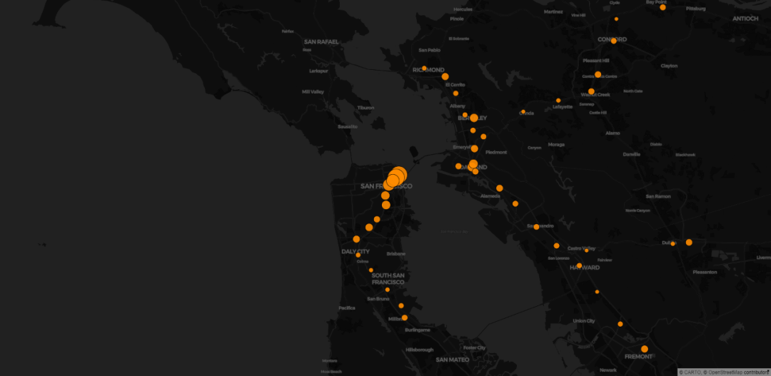
Figure of the number of exits of subway stations in San Francisco.

The code is as follows.

import pydeck as pdk
import pandas as pd
import math

SCATTERPLOT_LAYER_DATA = "https://raw.githubusercontent.com/visgl/deck.gl-data/master/website/bart-stations.json"
df = pd.read_json(SCATTERPLOT_LAYER_DATA)

# Use pandas to calculate additional data
df["exits_radius"] = df["exits"].apply(lambda exits_count: math.sqrt(exits_count))

# Define a layer to display on a map
layer = pdk.Layer(
    "ScatterplotLayer",
    df,
    pickable=True,
    opacity=0.8,
    stroked=True,
    filled=True,
    radius_scale=6,
    radius_min_pixels=1,
    radius_max_pixels=100,
    line_width_min_pixels=1,
    get_position="coordinates",
    get_radius="exits_radius",
    get_fill_color=[255, 140, 0],
    get_line_color=[0, 0, 0],
)

# Set the viewport location
view_state = pdk.ViewState(latitude=37.7749295, longitude=-122.4194155, zoom=10, bearing=0, pitch=0)

# Render
r = pdk.Deck(layers=[layer], initial_view_state=view_state, tooltip={"text": "{name}\n{address}"})
r.to_html("scatterplot_layer.html")

⑦ Other

There are many cases, so we don't post code here, just show it directly!

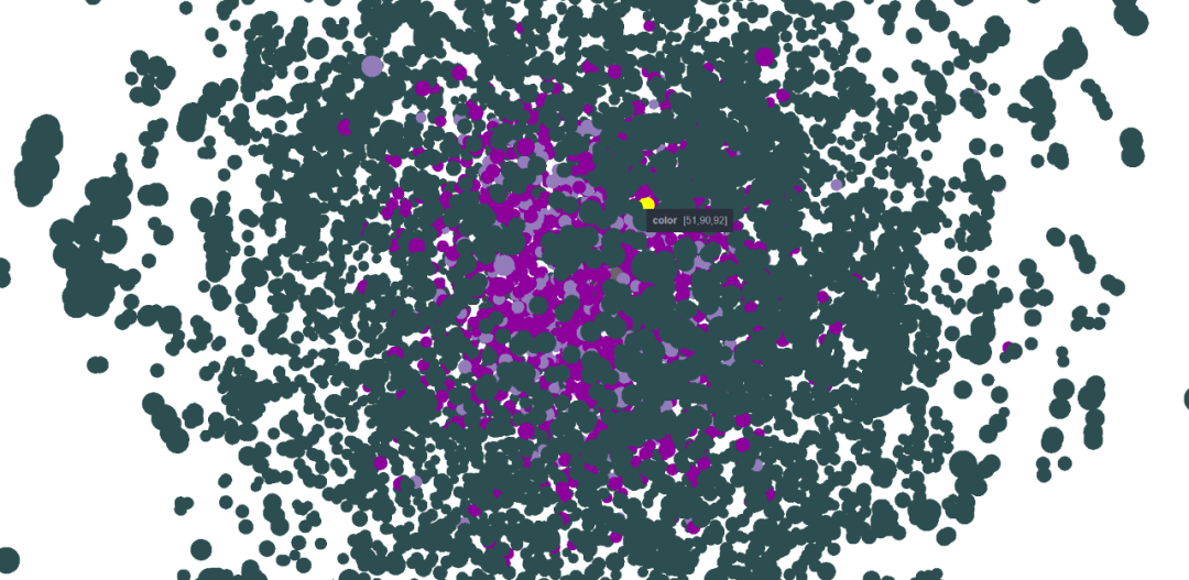
Rendered 10k points.

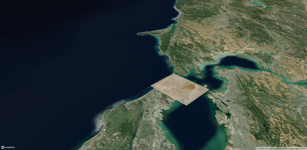
In 1906, Britton & Rey drew the fire map of San Francisco in 1906, covering the interactive map of San Francisco.

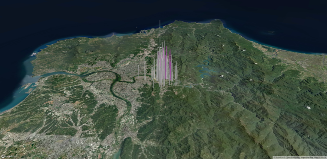
House prices in Taipei. The data is from 2012 to 2013. The height of the column indicates the rise of the price per unit area, and the color indicates the distance from the subway station.

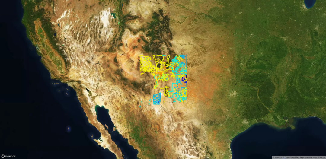
Location of livestock raised in New Mexico in 2006.

The position of poultry is blue and the position of cattle is orange. Superimposed with satellite images on Mapbox to highlight how terrain affects agriculture.

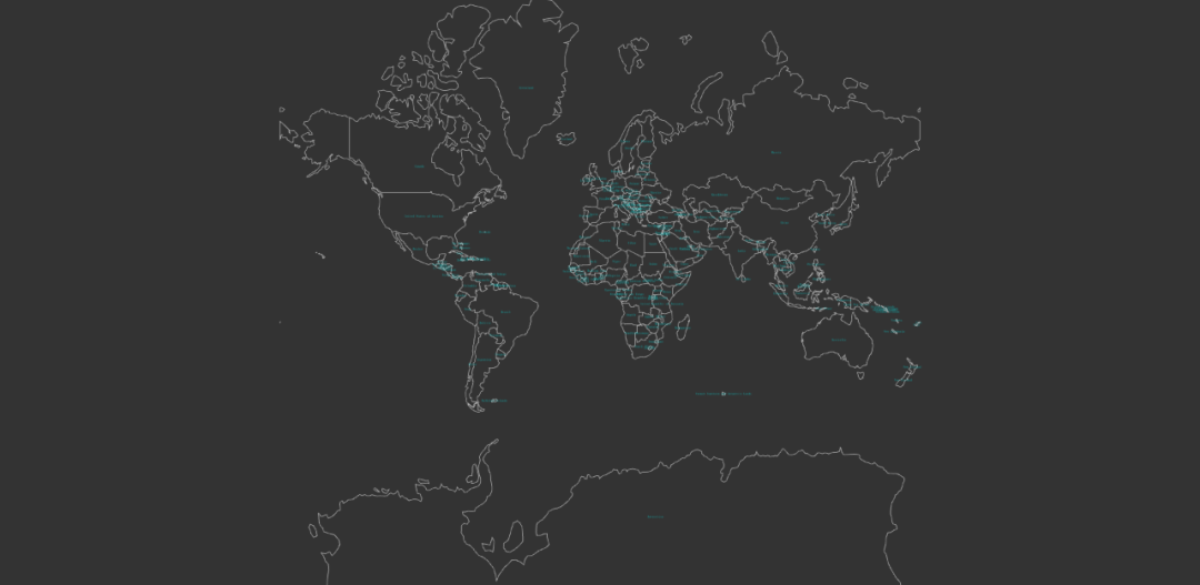
Universal style, a map of the world.

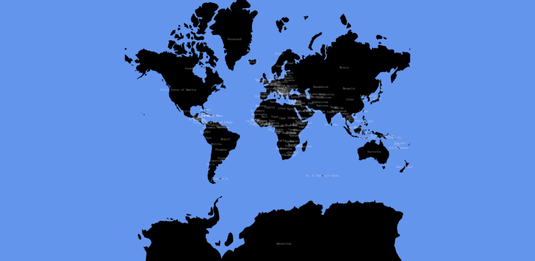
Draw the world map through the data of geopandas.

The installation of geopandas is a little laborious. It is recommended to use the whl installation package.

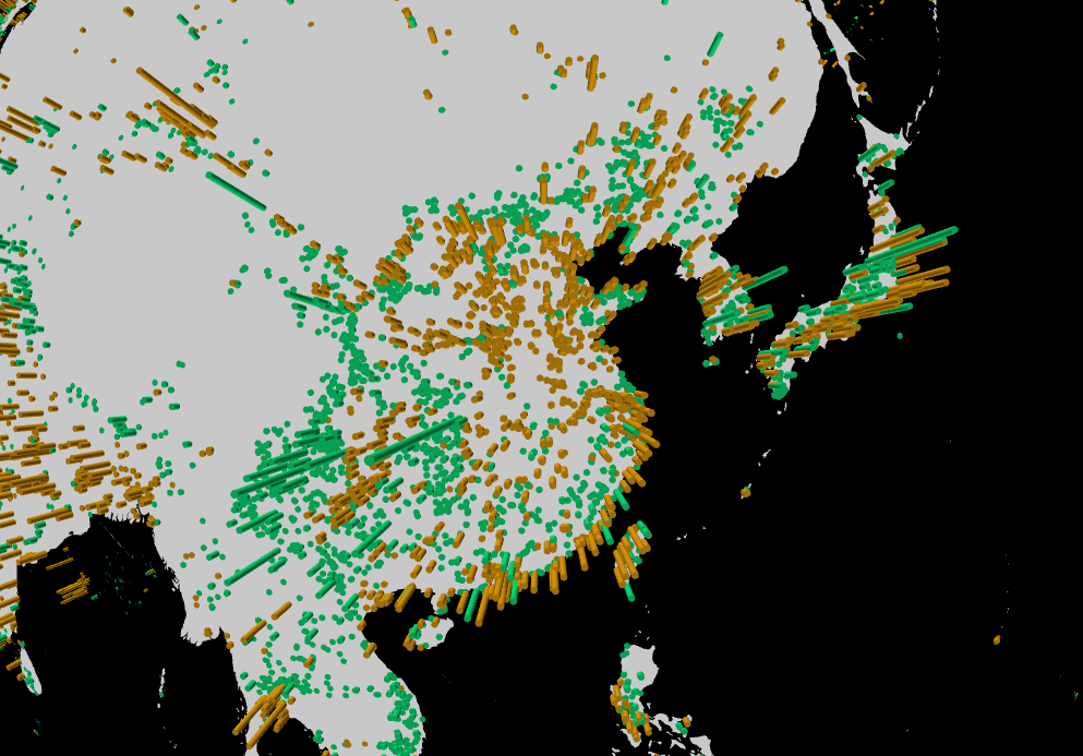
More than 33000 power plants in the world are mapped on a spherical map according to their production capacity (expressed in height) and fuel type (green, if renewable).

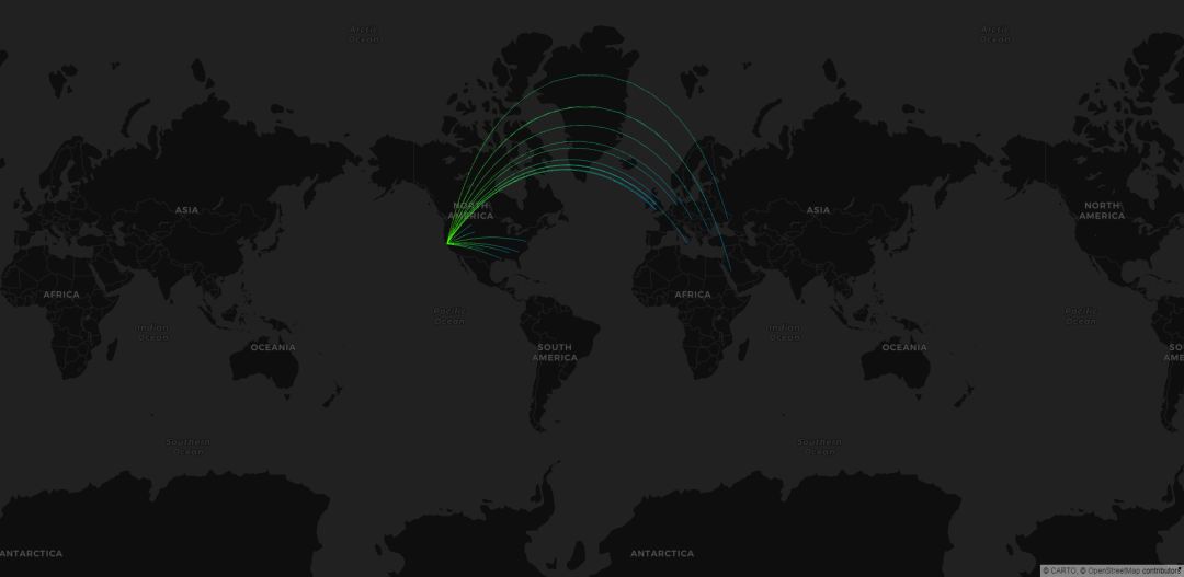
Direct flight route map of San Francisco International Airport. The starting point is green and the destination is blue.

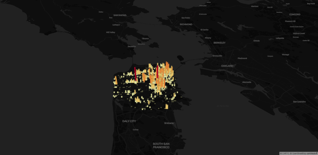
Distribution of bicycle parking places in San Francisco.

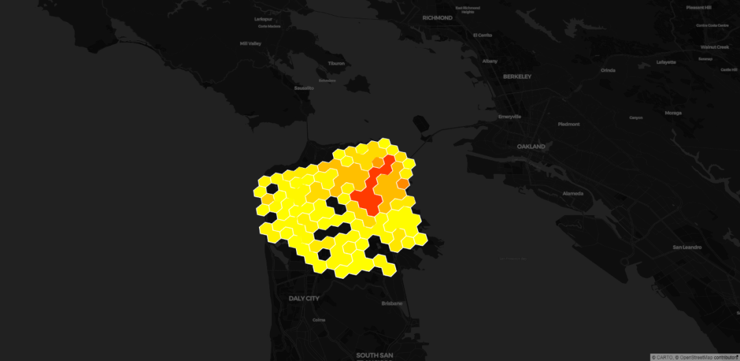
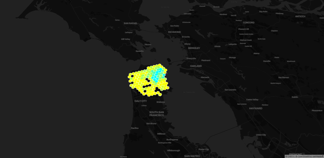
Grid map.

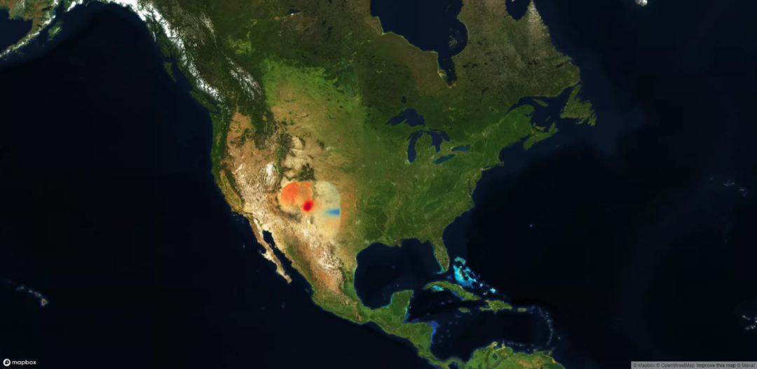
Location heat map of livestock raising in New Mexico in 2006.

The position of poultry is blue and the position of cattle is orange. Superimposed with satellite images on Mapbox to highlight how terrain affects agriculture.

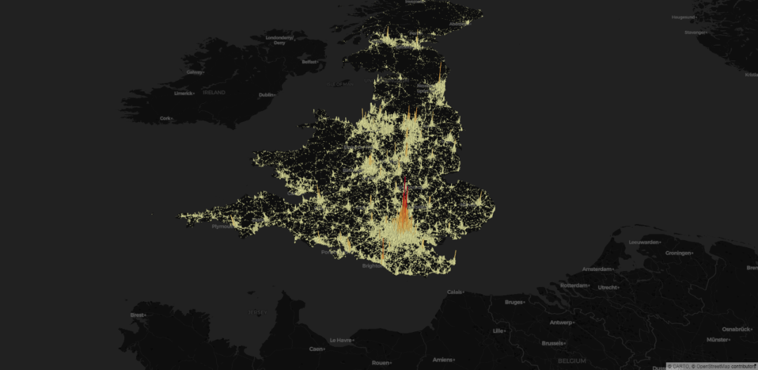
Personal injury and traffic accidents in Britain since 1979.

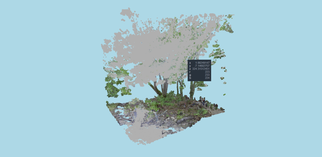
Point cloud image, laser scanning, composed of countless points.

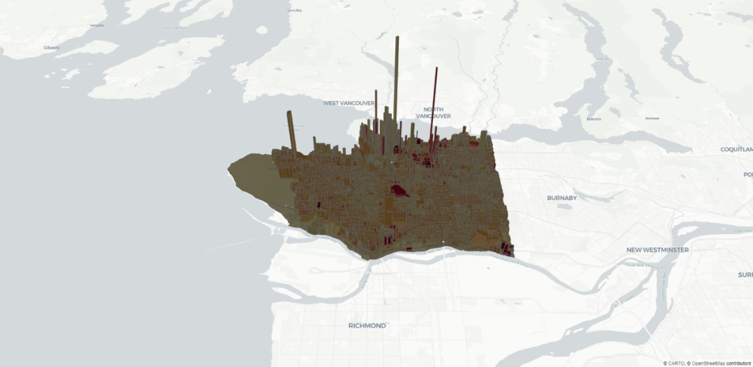
House prices in Vancouver, Canada.

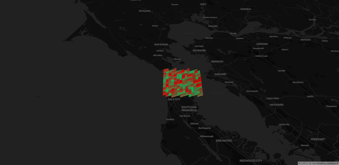
I don't know what this is

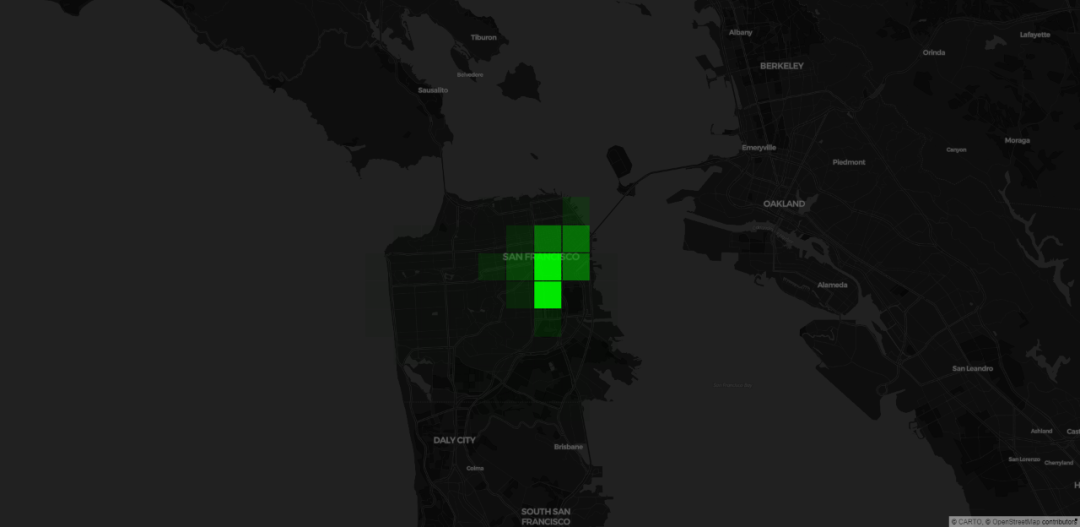
Bicycle parking spaces in San Francisco aggregate data into grids.

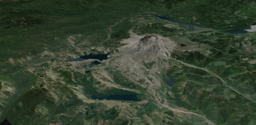
Create a topographic map using AWS open data and Mapbox satellite images.

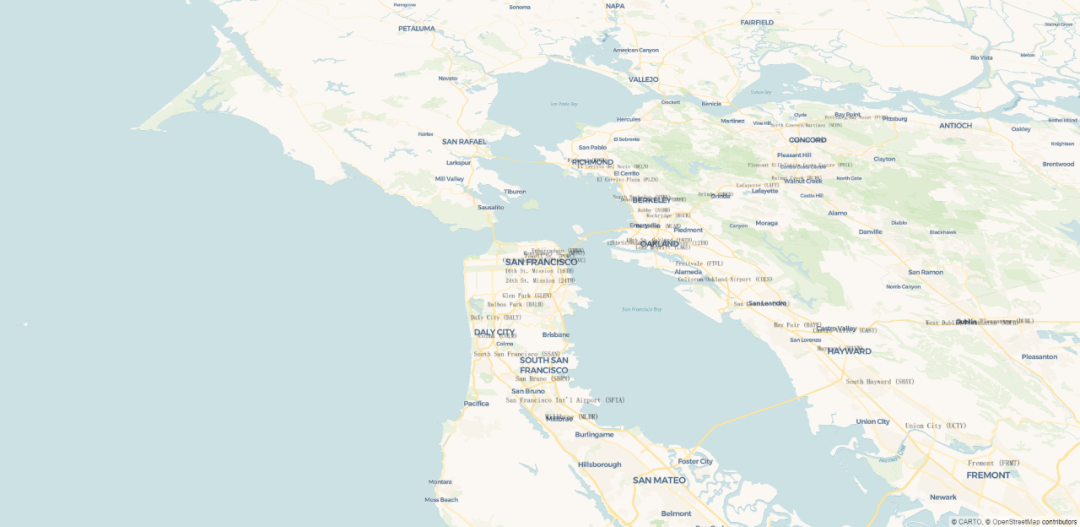
The names of various public transport stations in San Francisco are marked on the location of the stations.

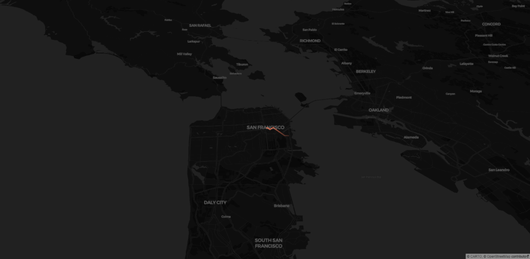
The riding of a shared bike in San Francisco gradually disappeared from the beginning.

Well, the above is the content shared today. You can practice by yourself.

Here, small F uses Mapbox map. It needs to register and obtain the token by itself.

Address:

https://account.mapbox.com/

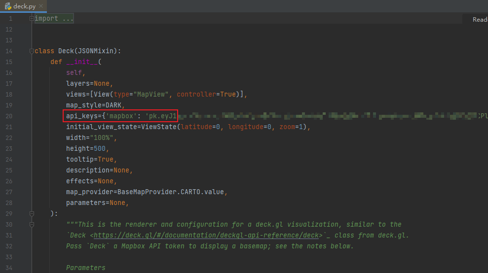
Then, in pydeck's deck method, add the token to the API_ The keys parameter is OK.