Reprint location: spatial transform network

In CNN classification, the locality, translation invariance, reduction invariance and rotation invariance of input samples need to be considered to improve the accuracy of classification. The essence of these invariance is the classical methods of image processing, that is, image clipping, translation, scaling and rotation, and these methods are actually spatial coordinate transformation of the image. One of the familiar spatial transformations is affine transformation. The affine transformation formula of the image can be expressed as follows:

Where, (xSource,ySourcexSource,ySource) represents the original image pixels, (xtarget, ytarget, xtarget, ytarget) represents the image pixels after affine transformation. coefficient matrix θθ That is, affine transformation coefficients, which can be adjusted by adjusting the coefficient matrix θθ， Realize the enlargement, reduction, translation and rotation of the image.

So, does the neural network have a way to realize these transformations adaptively with a unified structure? In this paper, a network model called Spatial Transform Networks (STN) is proposed. The network does not need the calibration of key points, and can adaptively transform and align the data according to classification or other tasks (including translation, scaling, rotation and other geometric transformations). When the spatial difference of input data is large, this network can be added to the existing convolution network to improve the accuracy of classification.

The main functions of the spatial transformation network proposed in this paper are:

1. The input can be transformed into the desired form of the next layer of the network;

2. It can automatically select the regional features of interest in the process of training;

3. It can realize the spatial transformation of various deformed data;

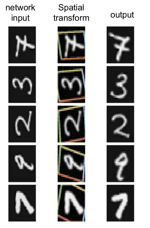
For example, for the handwritten font input in the figure above, we are interested in the area containing numbers in the yellow box. In the process of training, the learned spatial transformation network will automatically extract the local data features in the yellow box, and spatially transform the data in the box to obtain the output.

2. Detailed explanation of STN principle of spatial transformation network

The so-called spatial transformation network actually introduces a spatial transformation network between two layers of neural network. The spatial transformation network includes two parts. The network structure is shown in the following figure: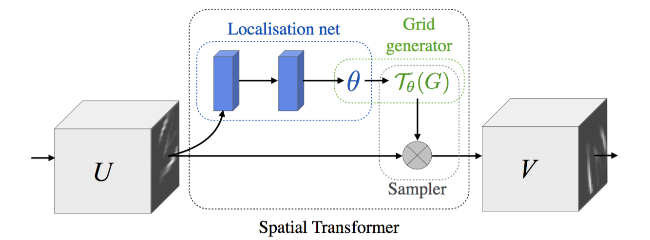

The first part is "localization net", which is used to generate affine transformation network structure, and the parameters in "localization net" network are the parameters that need to be trained in spatial transformation network;

The second part is spatial transformation, that is, affine transformation.

Affine transformation coefficients are generated through the local network θ (it can also be other types of spatial transformation, and the local network can be designed as needed to obtain the corresponding spatial transformation coefficients θ， This paper only takes affine transformation as an example to explain), and obtains affine transformation coefficients θ Then we can perform affine transformation on the input of the upper layer and input the affine transformation results to the next layer. For example, in the above figure, u is the feature map of an input image or a layer of CNN, V is the feature map after affine transformation, and the "spatial transformation network" is sandwiched between u and V. as mentioned above, "localization net" in this spatial transformation network is used to generate affine transformation coefficients θ，” "Localization net" can be a full connection layer or a volume layer. The specific network design needs to be set according to the actual needs. " "Localization net" to obtain affine transformation coefficients θ After that, we can affine transform the input u to get v. Finally, we will take the code as an example to explain the design of "localization net" network. Next, we will first talk about obtaining affine transformation coefficients θ The principle of affine transformation of U.

For affine transformation, if the affine transformation coefficient θ The output coordinate point (xTarget,yTarget) obtained by solving the input (xSource,ySource) is non integer, so it is necessary to consider the inverse affine transformation.

The so-called inverse affine transformation is to first generate the output coordinate grid points according to the output size of affine transformation, that is, the "Grid generator" in the above figure, for example, the size of V is 10 × At 10 o'clock, we can get a 10 × For the coordinate position point matrix of size 10, the next step is to perform affine transformation on the coordinate position point. The affine transformation formula and schematic diagram are as follows:

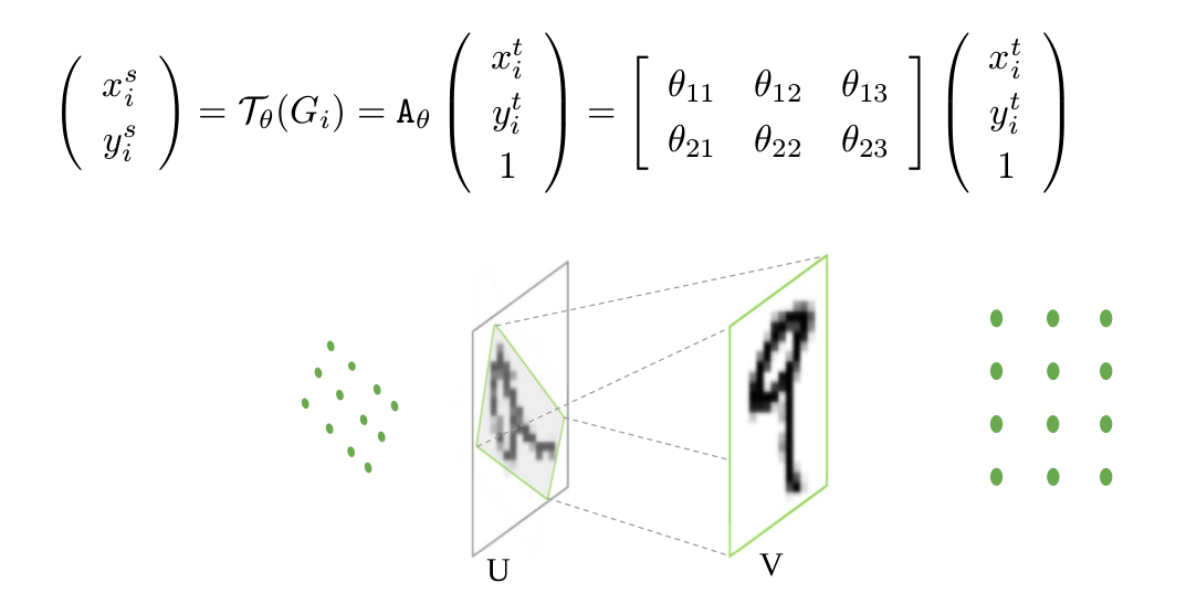
It should be noted that the affine coefficient at this time is θ After affine transformation, the corresponding position of the position coordinate point in V in u can be obtained. However, the coordinate points in U obtained at this time may still be non integers, so interpolation is usually required to obtain the corresponding coordinate points. After the coordinate points in u are obtained, they can be copied to V to obtain the affine transformation result v. The specific affine transformation process can also be understood in combination with the following figure: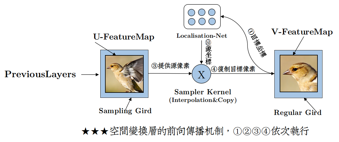

In the figure above, affine transformation coefficients are generated by Localisation Net θ After that, the process of affine transformation is to perform steps 1, 2, 3 and 4 in turn.

３. Practical application of spatial transformation network

The above explanation is the understanding of spatial transformation network. In practical application, how can we add spatial transformation network to our own network? Next, we will focus on the application of spatial transformation network.

3.1. Spatial transformation network is the first layer of the network

The spatial transformation network can be directly used as the first layer of the network, that is, the input of localization net is input, so as to directly perform affine transformation on the input. For the design of localization net, localization net can be designed as full connection layer or convolution layer according to the size of input. For example, for handwritten fonts, the input picture size is 40x40, that is, input=[batch_size,1600], Then we can design localization net to include two full connection layers. The first full connection layer w1=[1600,20],b1=[20], the first full connection layer w2=[20,6],b2=[6], and the output of the second full connection layer is [batch_size,6], which is the affine transformation coefficient. If the input size of the input localization net is large, it is necessary to add convolution and pooling layers in the localization net, and finally input it to the full connection layer to obtain the affine transformation coefficient; For the design of full connection layer and convolution layer, see reference codes 4.1 and 4.2.

3.2. The spatial transformation network is inserted into the middle layer of CNN

The spatial transformation network can also be added to the middle layer of CNN. The spatial transformation network can be directly inserted in front or behind the conv or max pooling layer. In addition, multiple spatial transformation networks can be inserted into the same layer of CNN. The network structure diagram of handwritten font inserted into CNN is given below: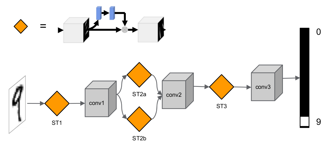

In the above figure, the first spatial transformation network ST1 acts on the input image and directly performs spatial transformation on the input image, the second and third spatial transformation networks st2a and st2b act on conv1 to perform spatial transformation on the convolution features of the first layer, and ST3 is used to perform spatial transformation on the convolution features of deeper layers.

Since the spatial transformation network can automatically extract local area features, inserting a parent spatial transformation network at the same layer of the network can extract multiple local area features, so it can be classified in combination with multiple local area features. For example, the network realizes the addition of handwritten fonts in two input pictures, and inserts two-layer spatial transformation network ST1 at the first layer of the network, ST2 and input its direct action language into the image. The third column in the figure shows the spatial transformation results. It can be seen from the figure that the networks ST1 and ST2 extract the features of different areas of the input handwritten font respectively.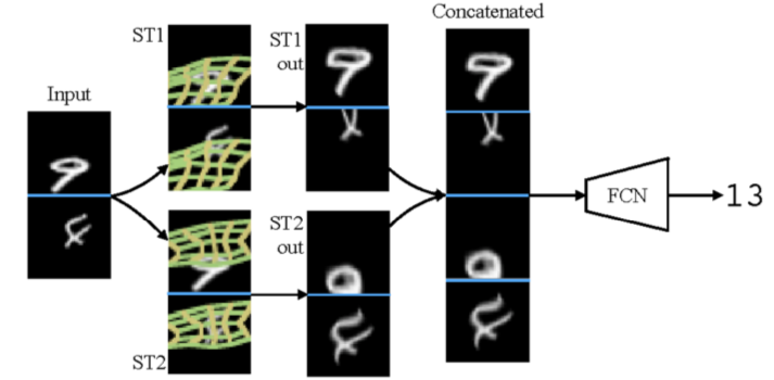

４. code analysis

First, let's take a look at the code implementation of affine transformation. As described above, the code is first implemented by the function_ meshgrid generates the coordinate position point grid of output V, and performs affine transformation on the grid through the affine transformation coefficient theta to obtain the position coordinate point t in U_ g. Then to T_g performs bilinear interpolation, and copies the pixel values of the coordinate points in the interpolated u into V to obtain the output v. The specific code is as follows:

    def transform(theta, input_dim, out_size):
        with tf.variable_scope('_transform'):
            num_batch = tf.shape(input_dim)[0]
            height = tf.shape(input_dim)[1]
            width = tf.shape(input_dim)[2]
            num_channels = tf.shape(input_dim)[3]
            theta = tf.reshape(theta, (-1, 2, 3))
            theta = tf.cast(theta, 'float32')

            # grid of (x_t, y_t, 1), eq (1) in ref [1]
            height_f = tf.cast(height, 'float32')
            width_f = tf.cast(width, 'float32')
            out_height = out_size[0]
            out_width = out_size[1]
            grid = _meshgrid(out_height, out_width)
            grid = tf.expand_dims(grid, 0)
            grid = tf.reshape(grid, [-1])
            grid = tf.tile(grid, tf.pack([num_batch]))
            grid = tf.reshape(grid, tf.pack([num_batch, 3, -1]))＃Get the output coordinate position point

            # Transform A x (x_t, y_t, 1)^T -> (x_s, y_s)
            T_g = tf.batch_matmul(theta, grid)#affine transformation 
            x_s = tf.slice(T_g, [0, 0, 0], [-1, 1, -1])#
            y_s = tf.slice(T_g, [0, 1, 0], [-1, 1, -1])
            x_s_flat = tf.reshape(x_s, [-1])
            y_s_flat = tf.reshape(y_s, [-1])

            input_transformed = _interpolate(
                input_dim, x_s_flat, y_s_flat,
                out_size)#Interpolation and output

            output = tf.reshape(
                input_transformed, tf.pack([num_batch, out_height, out_width, num_channels]))
            return output

Next, combined with two specific examples, we explain the design of "localization net" for full connection layer and convolution layer.

4.1 "localization net" is an example of the full connection layer:

In this example, the spatial transformation network is used to transform the input image. "localization net" includes two full connection layers. The specific network design is as follows:

    x = tf.placeholder(tf.float32, [None, 1600])#input
    y = tf.placeholder(tf.float32, [None, 10])


    x_tensor = tf.reshape(x, [-1, 40, 40, 1])


    W_fc_loc1 = weight_variable([1600, 20])#First full connection layer
    b_fc_loc1 = bias_variable([20])

    W_fc_loc2 = weight_variable([20, 6])#Second full connection layer

    initial = np.array([[1., 0, 0], [0, 1., 0]])
    initial = initial.astype('float32')
    initial = initial.flatten()
    b_fc_loc2 = tf.Variable(initial_value=initial, name='b_fc_loc2')


    h_fc_loc1 = tf.nn.tanh(tf.matmul(x, W_fc_loc1) + b_fc_loc1)

    keep_prob = tf.placeholder(tf.float32)
    h_fc_loc1_drop = tf.nn.dropout(h_fc_loc1, keep_prob)

    h_fc_loc2 = tf.nn.tanh(tf.matmul(h_fc_loc1_drop, W_fc_loc2) + b_fc_loc2)＃Affine transformation coefficient theta，Size bath_size*6

    out_size = (40, 40)
    h_trans = transformer(x_tensor, h_fc_loc2, out_size)

As shown in the code, the parameters to be trained in the spatial transformation network part are "localization net", including the parameters w of two full connection layers_ fc_ loc1， b_fc_loc1，W_fc_loc2， b_fc_loc2. The complete code link is as follows:
https:\/\/github.com\/tensorflow\/models\/blob\/master\/transformer\/cluttered_mnist.py

4.2 "localization net" is an example of a volume layer:

As shown in the following code, the "localization net" layer includes two convolution layers and two fully connected layers to obtain the affine transformation coefficient theta.

from keras.models import Sequential
from keras.layers.core import Dense, Dropout, Activation, Flatten
from keras.layers.convolutional import Convolution2D, MaxPooling2D

＃localization net,Affine transformation coefficients are obtained theta

locnet = Sequential()
locnet.add(MaxPooling2D(pool_size=(2,2), input_shape=input_shape))＃
locnet.add(Convolution2D(20, 5, 5))
locnet.add(MaxPooling2D(pool_size=(2,2)))
locnet.add(Convolution2D(20, 5, 5))

locnet.add(Flatten())
locnet.add(Dense(50))
locnet.add(Activation('relu'))
locnet.add(Dense(6, weights=weights))＃Output affine transformation coefficient theta
#locnet.add(Activation('sigmoid'))

＃build the model

model = Sequential()
model.add(SpatialTransformer(localization_net=locnet,
                             downsample_factor=3, input_shape=input_shape))#affine transformation 

model.add(Convolution2D(32, 3, 3, border_mode='same'))
model.add(Activation('relu'))
model.add(MaxPooling2D(pool_size=(2, 2)))
model.add(Convolution2D(32, 3, 3))
model.add(Activation('relu'))
model.add(MaxPooling2D(pool_size=(2, 2)))

model.add(Flatten())
model.add(Dense(256))
model.add(Activation('relu'))

model.add(Dense(nb_classes))
model.add(Activation('softmax'))

model.compile(loss='categorical_crossentropy', optimizer='adam')

The part to be trained in the localization net part is the coefficient of each layer of the locnet part. The complete code link is as follows:
(https://github.com/EderSantana/seya/blob/master/examples/Spatial%20Transformer%20Networks.ipynb)
 

--------
Copyright notice: This is the original article of CSDN blogger "imperfect00", which follows the CC 4.0 BY-SA copyright agreement. Please attach the original source link and this notice for reprint.
Original link: https://blog.csdn.net/u011961856/article/details/77920970