Chapter II
Section I data loading and preliminary observation
1.1 loading data
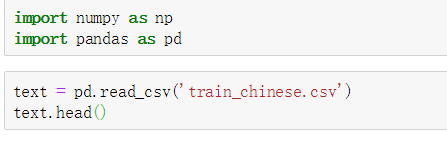
1.1.1 task 1: import numpy and pandas
import numpy as np
import pandas as pd
1.1.2 task 2: load data
(1) Load data using relative paths
#Import relative path data
df=pd.read_csv('train.csv')
(2) Load data using absolute path
#Absolute path import data
path=os.path.abspath('train.csv')
df = pd.read_csv(path)
extend
(1) Displays the number of table rows and columns
#Number of rows and columns
df.shape
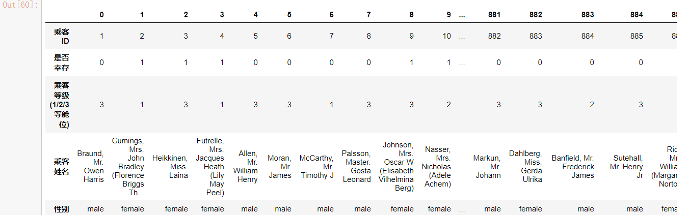
(2) Transpose table
#Transpose
df.T
Before transpose
After transposition
(3)read_table has no separation by default
#No delimited data
pd.read_table(path)
read_csv is separated by commas by default, and table is separated by commas. You need to set parameters
#Comma separator
pd.read_table(path,sep=',')
1.1.3 task 3: read one data module every 10 rows block by block
#Block by block reading
df = pd.read_csv('train.csv',chunksize=10)
df.get_chunk()
Block by block reading is to truncate the reading analysis of long files.
Comparison of block by block read type and non block by block read type:
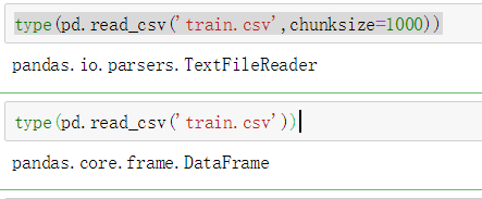
Block by block reading is not allowed for head display.
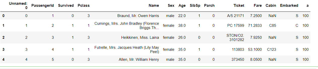
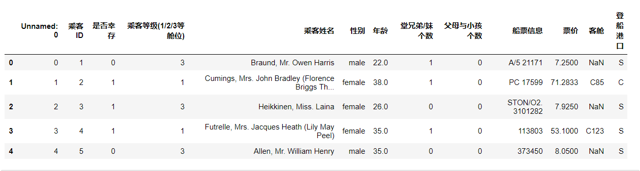
1.1.4 task 4: change the header to Chinese and the index to passenger ID [for some English materials, we can get familiar with our data more intuitively through translation]
Passengerid = > passenger ID
Survived = > survived
Pclass = > passenger class (Class 1 / 2 / 3)
Name = > passenger name
Sex = > gender
Age = > age
Sibsp = > number of cousins / sisters
Parch = > number of parents and children
Ticket = > ticket information
Fare = > fare
Cabin = > cabin
Embarked = > port of embarkation
The first method:
#Change header to Chinese
df.columns = ['passenger ID','Survive','Passenger class(1/2/3 Class space)','Passenger name','Gender','Age','male cousins/Number of sisters','Number of parents and children','Ticket information','Ticket Price','passenger cabin','Boarding port']
The second method:
#Other methods: add one more line
df = pd.read_csv('train.csv',names=['passenger ID','Survive','Passenger class(1/2/3 Class space)','Passenger name','Gender','Age','male cousins/Number of sisters','Number of parents and children','Ticket information','Ticket Price','passenger cabin','Boarding port'])
df
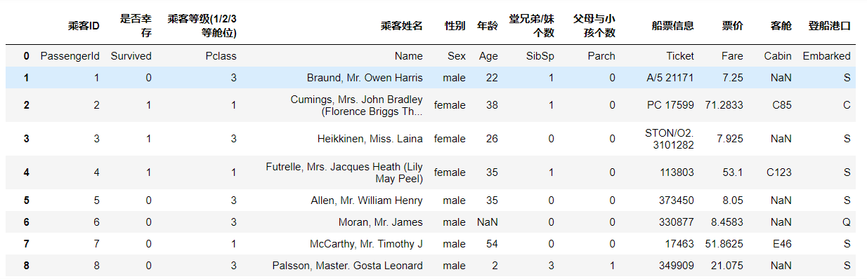
Change the name when reading the file, and add an additional column at the end. The previous list name becomes a row in it. This method is generally not adopted. (easily confused data)
1.2 preliminary observation
1.2.1 task 1: View basic information of data
give an example:
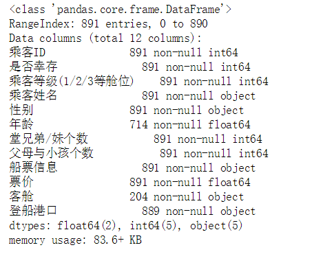
#1. View basic data information
df.info()
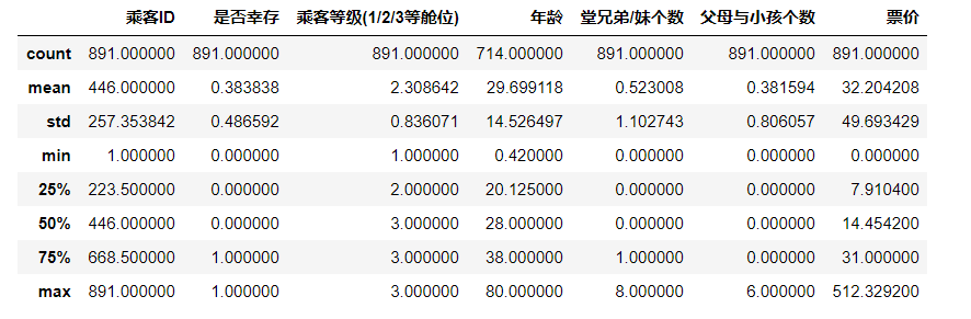
#2. View basic information
df.describe()
#mean std standard deviation
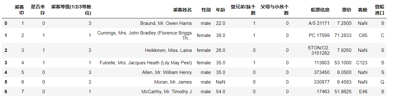
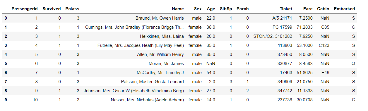
1.2.2 task 2: observe the data in the first 10 rows and the data in the last 15 rows of the table
head() and tail() display 5 columns by default.
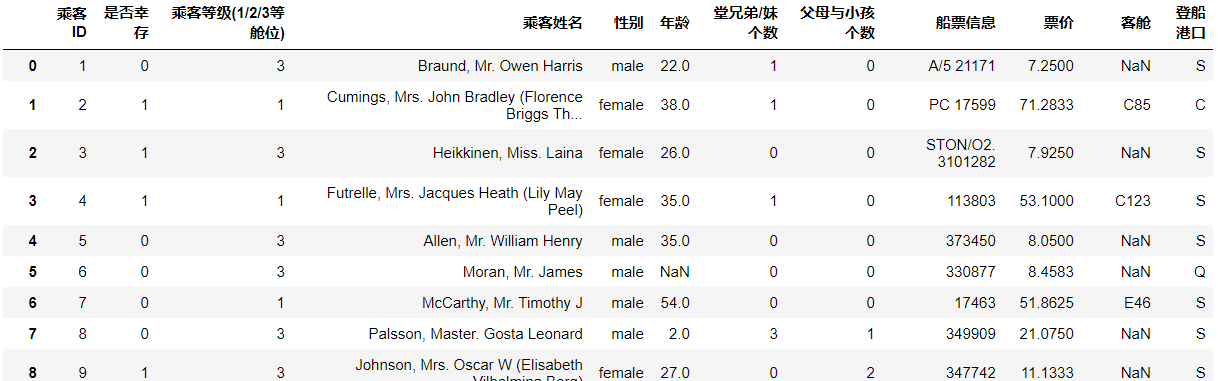
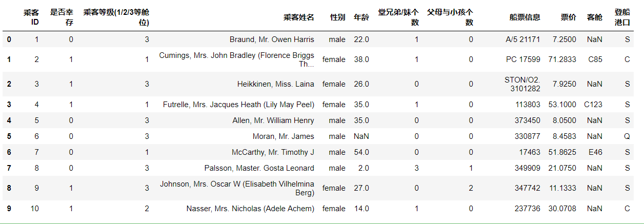
#Observe the data in the first 10 rows of the table
df.head(10)
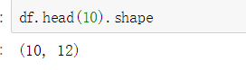
#Observe the data in the last 15 rows of the table
df.tail(15)
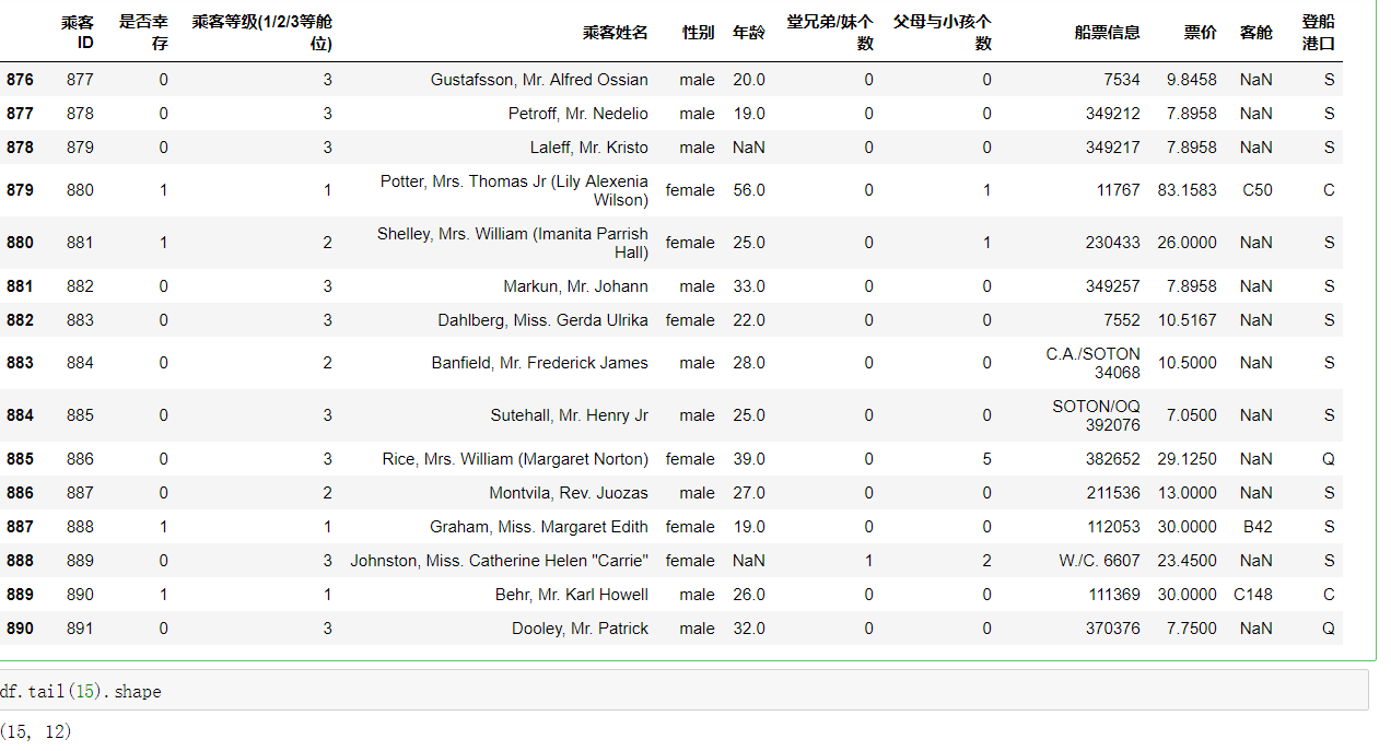
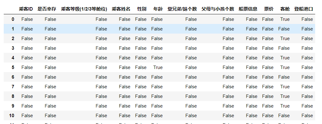
1.2.4 task 3: judge whether the data is empty, return True where it is empty, and return False in other places
#Judge whether the data is empty, return True where it is empty, and return False in other places
df.isnull()
1.3 saving data
1.3.1 task 1: save the data you loaded and changed as a new file train in the working directory_ chinese. csv
df.to_csv('train_chinese.csv')
Section II pandas Foundation
1.4 know what your data is
1.4.1 task 1: there are two data types in pandas, DateFrame and Series. You can simply understand them by searching. Then write a small example about these two data types 🌰 [open question]
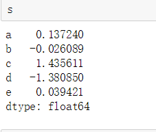
Series
First example:
#Series one-dimensional array type with index, random gets random number
s=pd.Series(np.random.randn(5),index=['a','b','c','d','e'])
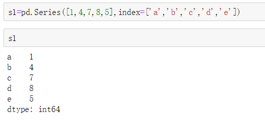
Second example:
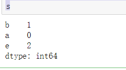
The third example:
#Dictionary form
s=pd.Series({'b':1,'a':0,'e':2})
s
DataFrame
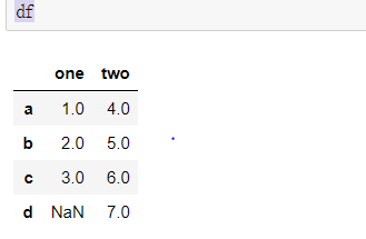
The fourth example:
#DataFrame two-dimensional array, which can be generated by Series
d = {'one' : pd.Series([1.,2.,3.],index=['a','b','c']),'two': pd.Series([4.,5.,6.,7.],index=['a','b','c','d'])}
df = pd.DataFrame(d)
df
1.4.2 task 2: load the "train.csv" file according to the method of the previous lesson
Relative path introduction is used here.
df=pd.read_csv('train.csv')
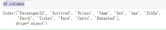
1.4.3 task 3: view the name of each column of DataFrame data
df.columns
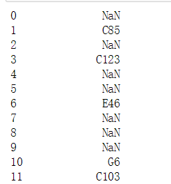
1.4.4 task 4: check all values in the "bin" column [there are many methods]
1.4.4 Task 4: View"Cabin"All values in this column [There are many ways]
The first method:
df.Cabin
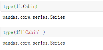
The second method:
df['Cabin']

Type view:
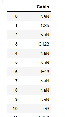
Can become DataFrame type:
#Become DataFrame type
df[['Cabin']]
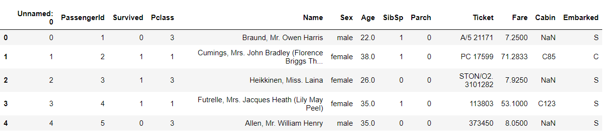
1.4.5 task 5: load the file "test_1.csv", then compare "train.csv" to see what extra columns are, and then delete the extra columns
Load the file "test_1.csv"
test_1 = pd.read_csv('test_1.csv')
test_1.head()
You can find that column a is redundant. Delete the extra column a:
The first way:
#Delete extra columns
del test_1['a']
test_1.head()
The second way:
test_1.pop('a')
test_1.head()
The third way:
#A copy of the array of deleted columns is generated, and the file itself does not delete columns
test_1.drop(['a'],axis=1)
The fourth way:
#Do not return the copy, save it directly into the original file
test_1.drop(['a'],axis=1,inplace = True)
test_1.head()
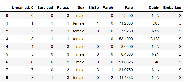
1.4.6 task 6: hide the ['PassengerId', 'Name', 'Age', 'Ticket] column elements, and only observe the other column elements
#Column element hiding
test_1.drop(['PassengerId','Name','Age','Ticket'],axis=1)
1.5 logic of screening
1.5.1 task 1: we take "Age" as the screening condition to display the information of passengers under the Age of 10.
#Displays information about passengers under the age of 10
df[df["Age"]<10]
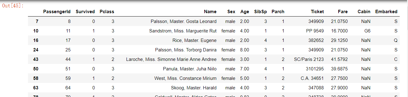
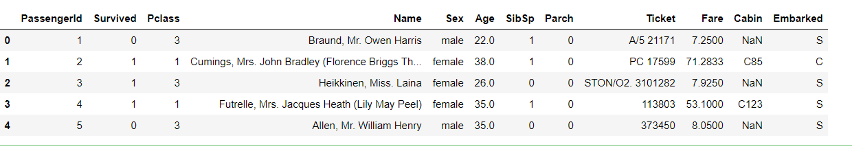
1.5.2 task 2: display the information of passengers aged over 10 and under 50 under the condition of "Age", and name the data as middle
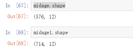
#The information of passengers aged over 10 and under 50 is displayed, and the data is named middle
midage = df[(df["Age"]>10)& (df["Age"]<50)]
midage.head()
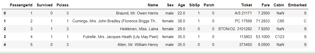
midage1 = df[(df["Age"]>10)|(df["Age"]<50)]
midage1.head()
Differences between comparison & and filtering data:
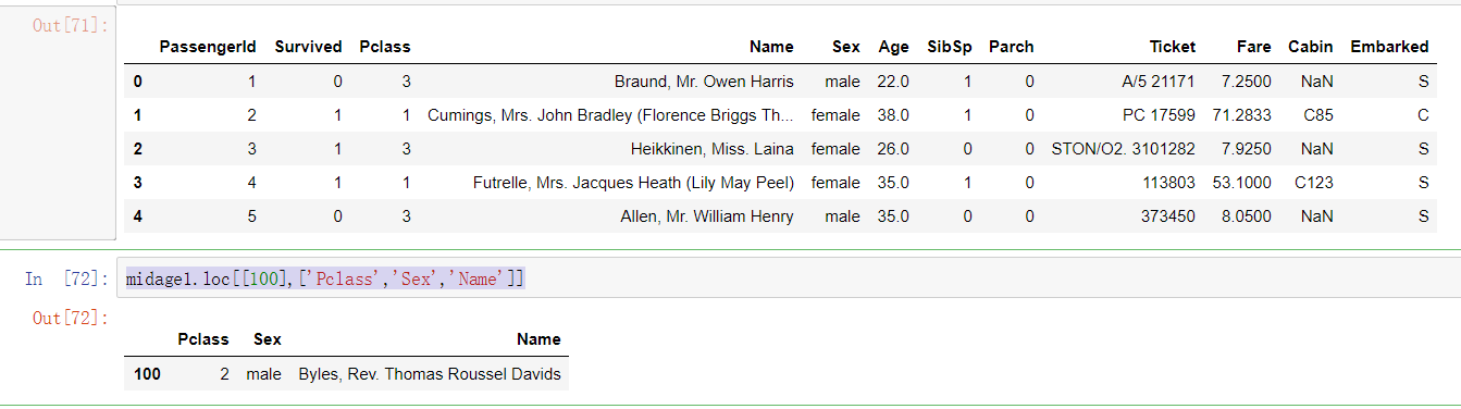
1.5.3 task 3: display the data of "Pclass" and "Sex" in the 100th row of middle data
#No reset_index will cause an index error and find the original data index 100 instead of the 100th row in the middle
midage.loc[[100],['Pclass','Sex','Name']]
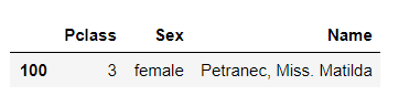
midage1 = midage.reset_index(drop=True)
midage1.head()
midage1.loc[[100],['Pclass','Sex','Name']]
We can compare the two indexes to see the problem:
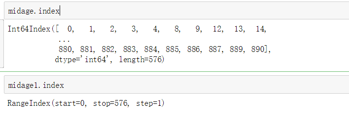
As we can see, without reset_index will cause an index error and find the original data index number instead of the index number in the set middle
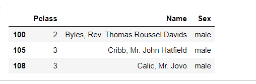
1.5.4 task 4: use the loc method to display the data of "Pclass", "Name" and "Sex" in line 100105108 of the middle data
#Use the loc method to display the data of "Pclass", "Name" and "Sex" in line 100105108 of the middle data
midage1.loc[[100,105,108],['Pclass','Name','Sex']]
1.5.5 task 5: use iloc method to display the data of "Pclass", "Name" and "Sex" in line 100105108 of middle data
#iloc index
#Use the iloc method to display the data of "Pclass", "Name" and "Sex" in line 100105108 of the middle data
midage1.iloc[[100,105,108],[2,3,4]]
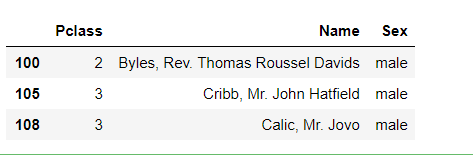
The comparison shows that when iloc method is used, the parameter is the index number of its column.
Section III exploratory data analysis
Import the required packages and data first:
1.6 do you know your data?
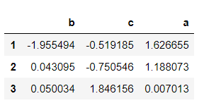
1.6.1 task 1: use Pandas to sort the sample data in ascending order
#Ascending sort
sample= pd.DataFrame(np.random.randn(3, 3),
                     index=list('213'),
                     columns=list('bca'))
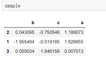
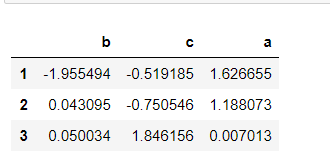
#Sort a column from small to large
sample.sort_values('b')
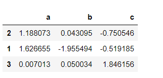
# Make row index sort ascending
sample.sort_index()
# Sort column index in ascending order
sample.sort_index(axis=1)
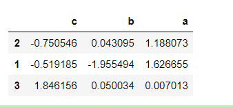
# Sort column index in descending order
sample.sort_index(axis=1, ascending=False)
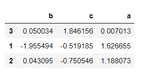
# Let any two columns of data be sorted in descending order at the same time. If it is impossible to sort at the same time, the first column in by will be selected first
sample.sort_values(by=['c', 'a'], ascending=False)
1.6.2 task 2: comprehensively sort the Titanic data (trian.csv) by fare and age (in descending order). What can you find from the data
#The Titanic data (trian.csv) is comprehensively sorted by ticket price and age (in descending order)
text.sort_values(by=['Ticket Price','Age'], ascending=False)
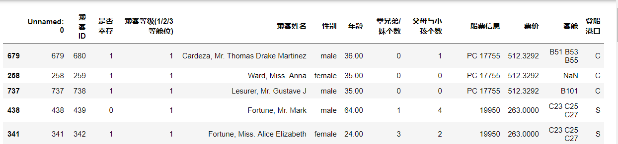
It is found that priority is given to ranking according to ticket prices, and then ranking on the basis of ticket prices according to age. And the higher the ticket price, the lower the mortality rate, among which none of the people with the highest ticket price died.
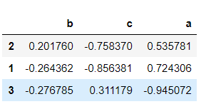
1.6.3 task 3: use Pandas to perform arithmetic calculation and calculate the data addition result of two dataframes
#Use Pandas for arithmetic calculation and calculate the data addition result of two dataframes
x= pd.DataFrame(np.random.randn(3, 3),
                     index=list('213'),
                     columns=list('bca'))
x
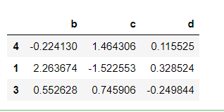
y= pd.DataFrame(np.random.randn(3, 3),
                     index=list('413'),
                     columns=list('bcd'))
y
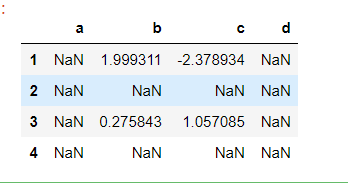
#Only when the rows and columns are the same can the calculation result be obtained
x+y
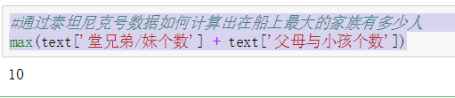
1.6.4 task 4: how to calculate the number of the largest family on board through the Titanic data?
#How to calculate the number of the largest family on board from the Titanic data
max(text['male cousins/Number of sisters'] + text['Number of parents and children'])
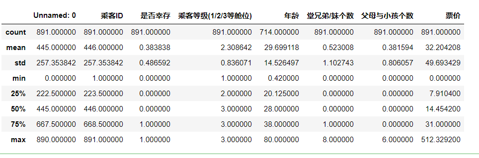
1.6.5 task 5: learn to use the Pandas describe() function to view basic statistics of data
#Use the Pandas describe() function to view the basic statistics of data. The first section has been run
text.describe()
The data display is not very intuitive. We can introduce histogram to see:
#Draw histogram
from matplotlib import pyplot as plt
#Pay attention to whether there is a blank value. If there is a blank value, an error will be reported, such as age
plt.hist(text['Survive'])
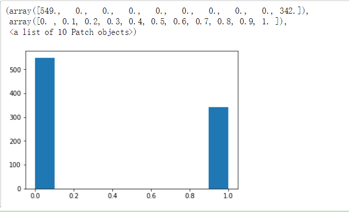
Using the histogram, we can clearly see the number of survivors and the number of deaths.
1.6.6 task 6: look at the basic statistics of ticket prices, parents and children in the Titanic data set. What can you find?
First, let's analyze the ticket price:
text['Ticket Price'].describe()
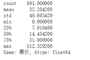
The average ticket price is 32 yuan, but the maximum ticket price is 512 yuan. We can still use charts to observe.
plt.hist(text['Ticket Price'])
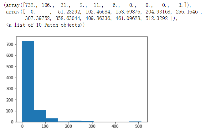
We can find that the ticket price distribution has a long tail.
The number of parents and children is analyzed below:
text['Number of parents and children'].describe()
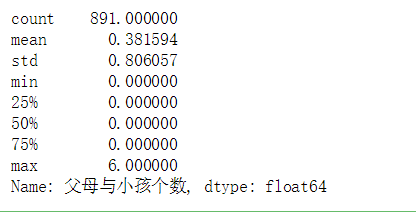
We can also see that his distribution has a long tail, with an average number of 0.38 But the maximum number is 6. The following is a visual representation of the histogram:
plt.hist(text['Number of parents and children'])
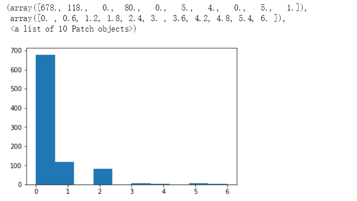
We can clearly see that most people travel alone.
[summary]
In this chapter, we make a preliminary statistical view of the data through the operation of the basic function, and gradually build the thinking of how to analyze the data.