api import:
import pandas as pd
import numpy as np
from sklearn.linear_model import LogisticRegression as LR
Data acquisition:
df = pd.read_csv('./Data/rankingcard.csv',index_col=0)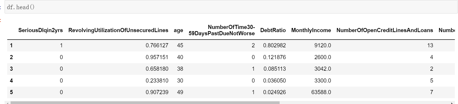
Remove duplicates:
When you manually enter or enter more than one line, duplicate data is likely to appear. You need to remove the duplicate values first,
# Remove duplicate values
df.drop_duplicates(inplace=True) # drop_duplicates removes duplicate values
After removing duplicate values, the data is deleted, but the index does not change. At this time, you need to reset the index value.
df.index = range(df.shape[0])
Missing value handling:
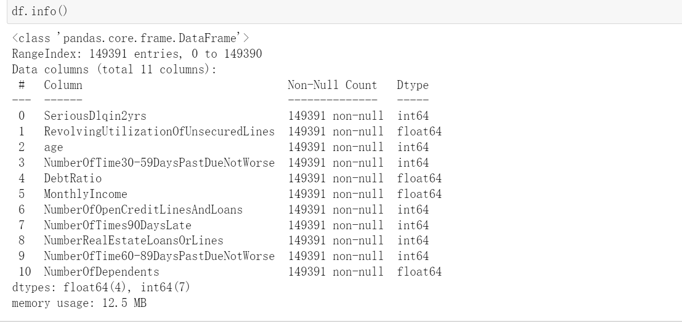
df.isnull().mean()
# It can be seen here that the number of families has a missing value of about% 2, and the income has a missing value of about 20%. During the credit evaluation, the impact of monthly income is too large, and there will be no large number of missing in the actual situation. Here, random forest is used to fill in

Fill in less missing features with averages:
# Average number of households filled
df.loc[:,'NumberOfDependents'].fillna(df.loc[:,'NumberOfDependents'].mean(),inplace=True)
Income has a great impact on the results, and there are many missing data. Here, random forest is used to fill in the missing value of income:
x = data.loc[:,data.columns != 'MonthlyIncome']

y = data.loc[:, 'MonthlyIncome']

# Split dataset
y_train = y[y.notnull()]
y_test = y[y.isnull()]
x_train = x.iloc[y_train.index,:]
x_test = x.iloc[y_test.index,:]

from sklearn.ensemble import RandomForestRegressor
rf = RandomForestRegressor()
rf.fit(x_train,y_train)

y_pre = rf.predict(x_test)

df.loc[df.loc[:,'MonthlyIncome'].isnull(),'MonthlyIncome'] = y_pre
Missing value resolution!
Exception handling:
# outlier handling -- box diagram, 3seigma rule, descriptive statistical observation to deal with outliers. Descriptive rule is used here
Observation data:
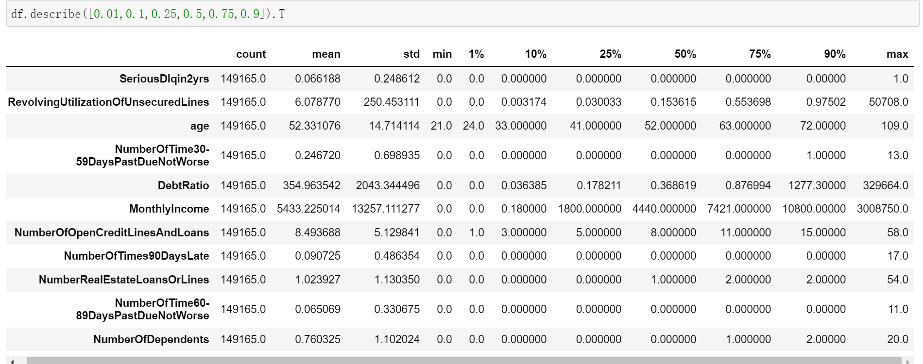
#The observed data will have two outliers
#Age here, there is a minimum value of zero, which is obviously unreasonable
#Then, the number of days of default here, 30 ~ 59,60 ~ 89,90 days overdue within two years, has a maximum of 98 times, which is an impossible thing to do
#In actual work, you can ask the data source workers about the situation and ask them how to calculate it. Here, we directly deal with it as an abnormal value
# Delete age anomalies
df = df[df['age'] != 0]

# Delete overdue exceptions
df = df[df['NumberOfTime30-59DaysPastDueNotWorse'] < 90]

# When deleting data, you must redefine the index
df.index = range(df.shape[0])
According to the above descriptive statistics, the data dimensions are obviously inconsistent, but there is no data standardization processing here. Although the data obey the normal distribution, the gradient decline can converge faster, our ultimate goal is to serve the business. The score card is a card used by business personnel to score customers based on various information filled in by new customers, Once the data is unified, the size and scope of the data will change, which may not be understood by business personnel. Therefore, due to business needs, we try our best to keep the original appearance of the data.
imblearn handles sample imbalance:
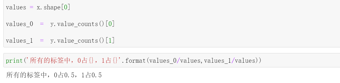
import imblearn
#imblearn is a library specially used to deal with unbalanced data sets. Its performance is much better than sklearn in dealing with sample imbalance
#imblearn is also a class by class, which also needs to be instantiated and fit, which is similar to sklearn

from imblearn.over_sampling import SMOTE

sm = SMOTE(random_state = 22)

x,y = sm.fit_resample(x,y)

y.value_counts()
Here to complete data preprocessing: 1 duplicate value processing, 2 missing value processing, 3 abnormal value processing, 4 sample imbalance processing
Divided into training set and test set:
#Divide training set and test set - when dividing the box (different scores are established in each stage), we need a structure of feature matrix and label. After dividing the data set, we can combine the training set and test set respectively
y = pd.DataFrame(y)

x = pd.DataFrame(x)

x_train,x_test,y_train,y_test = train_test_split(x,y,test_size=0.2,random_state=22)

model_data = pd.concat([y_train,x_train],axis=1)
test_data = pd.concat([y_test,x_test],axis=1)

model_data.index = range(x_train.shape[0])
test_data.index = range(x_test.shape[0])

model_data.to_csv('./Data/model_data.csv')
test_data.to_csv('./Data/test_data.csv')
#The core part of the score card -- sub box
#Classify each feature to facilitate the staff's scoring
#The core is to discretize continuous data, so the number of boxes should not be too large,
#To understand a concept, the discretization of continuous variables must be accompanied by the loss of information. The fewer boxes, the greater the loss of information
#IV to measure the amount of information on features and the contribution of features to the prediction function
#Box splitting idea: WOE (weight of evidence) bad% (proportion of bad customers)
#1) We first divide the continuous variables into a group of categorical variables with a large number, for example, divide tens of thousands of samples into 100 groups or 50 groups
#2) Ensure that each group contains samples of two categories, otherwise the IV value will not be calculated
#3) We perform chi square test on adjacent groups. Groups with large P value (weak correlation) in Chi square test are merged until the number of groups in the data is less than the set N box
#4) Let's divide a feature into [2,3,4..... 20] boxes respectively, observe how the IV value changes under the number of boxes, and find out the most suitable number of boxes (let N from 2 to 20, and draw a learning curve of boxes)
#5) After the boxes are divided, we calculate the WOE value of each box, bad%, and observe the effect of boxes
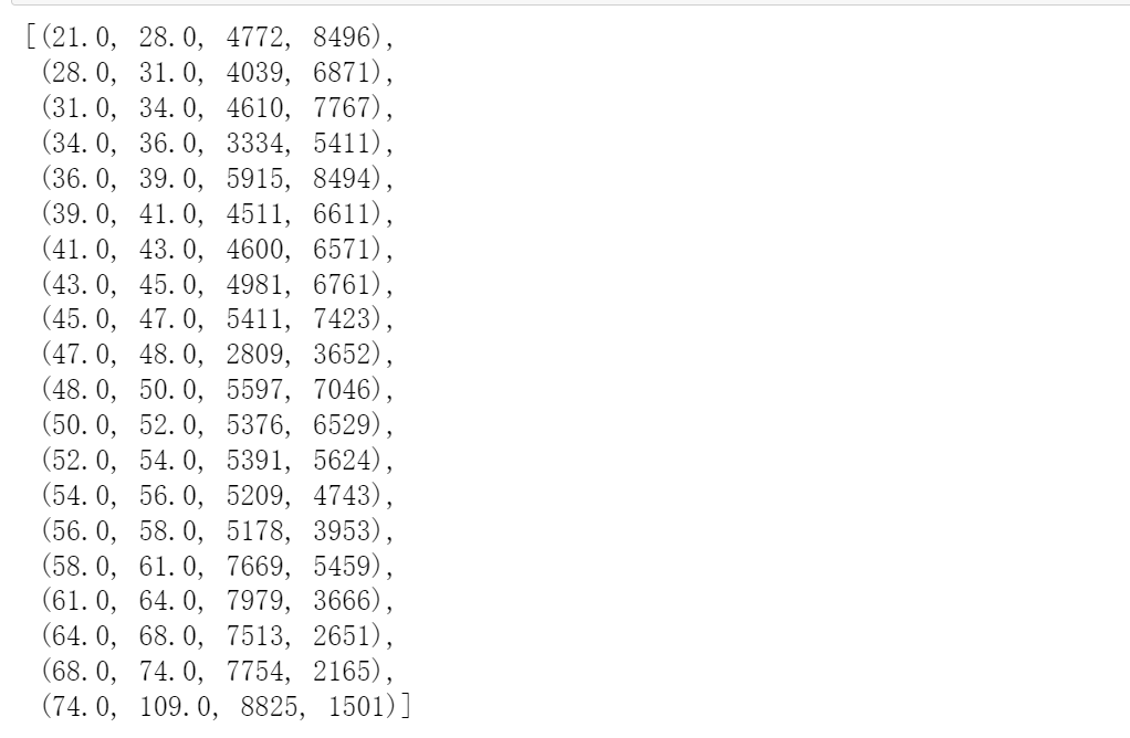
model_data['qcut'],updown = pd.qcut(model_data['age'],retbins=True,q=20,duplicates='drop')
"""
pd.qcut,The essence of quantile based box function is to discretize continuous variables
 Only one-dimensional data can be processed. Returns the upper and lower limits of the box
 parameter q: Number of boxes to be divided
 parameter retbins=True At the same time, the return structure is the index, the sample index and the element is the index of the assigned box Series(Which box does this element belong to)
Now return two values: which box each sample belongs to, and the upper and lower limits of all boxes
"""
# Group aggregation calculates the number of 0 and 1 in the distribution box.
count_0 = model_data[model_data['SeriousDlqin2yrs'] == 0].groupby(by='qcut').count()['SeriousDlqin2yrs']
count_1 = model_data[model_data['SeriousDlqin2yrs'] == 1].groupby(by='qcut').count()['SeriousDlqin2yrs']

# Pack the upper and lower limits of each box, the number of 0 and the number of 1 together
num_bins = [*zip(updown,updown[1:],count_0,count_1)]
#Calculate WOE and BAD RATE
#BAD RATE and bad% are not the same thing
#BAD RATE is the proportion of bad samples in a box (bad/total)
#Bad% is the proportion of bad samples in a box in the whole feature
def get_woe(num_bins):

    column = ['min','max','count_0','count_1']

    num_bin = pd.DataFrame(num_bins,columns=column)

    num_bin['total'] = num_bin.count_0 + num_bin.count_1

    num_bin['bad_rate'] = num_bin.count_1/num_bin.total

    num_bin['percentage'] = num_bin.total/num_bin.total.sum()

    num_bin['bad'] = num_bin.count_0/num_bin.count_0.sum()

    num_bin['good'] = num_bin.count_1/num_bin.count_1.sum()

    num_bin['woe'] = np.log(num_bin['good']/num_bin['bad'])

    return num_bin
def get_iv(num_bin):
rate = num_bin['good'] - num_bin['bad']
iv = np.sum(rate * num_bin.woe)
return ivThe calculated iv value is:
0.36095534222757264
After writing out the corresponding function, carry out chi square test, merge the box and draw the iv curve.
# Calculate the maximum p value
iv_nums = []
axisx = []
while len(num_bins_) > 2: # Here n stands for the number of boxes to determine how many boxes to divide
pvs = []
for j in range(len(num_bins_)-1):
pv = scipy.stats.chi2_contingency([num_bins_[j][2:],num_bins_[j+1][2:]])[1]
pvs.append(pv)
i = pvs.index(max(pvs))
# Observe the index where the maximum p value is located and determine that it is num_bins_ Generated from the first and second columns of data (starting from zero),
# Merge the first column and the second column. The beginning of the merged data is the beginning of the first column, and the end is the end of the second column. The amount of tree with label equal to 0,1 is the sum of the two columns
num_bins_[i:i+2]= [(
num_bins_[i][0],
num_bins_[i+1][1],
num_bins_[i][2]+num_bins_[i+1][2],
num_bins_[i][3]+num_bins_[i+1][3])]
axisx.append(len(num_bins_))
iv_nums.append(get_iv(get_woe(num_bins_)))
plt.figure(figsize=(20,8),dpi=100)
plt.plot(axisx,iv_nums)
plt.xticks(axisx)
plt.show()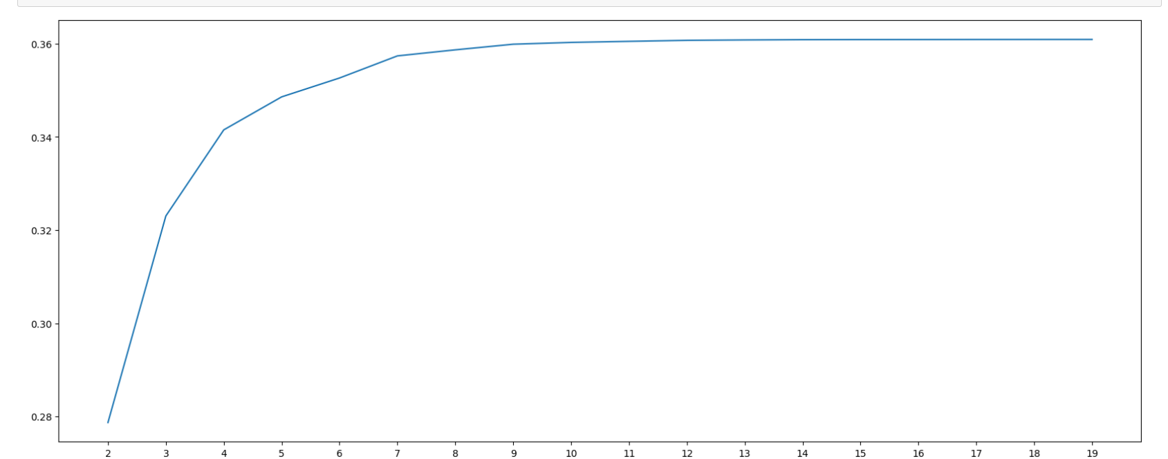
Because the fewer boxes themselves will lead to greater information loss, we observe the image and choose the direction in which the image drops the fastest 6
Use the best number of boxes to verify the results
# Define a box function
def get_bin(num_bins_,n):
while len(num_bins_) > n: # Here n stands for the number of boxes to determine how many boxes to divide
pvs = []
for j in range(len(num_bins_)-1):
pv = scipy.stats.chi2_contingency([num_bins_[j][2:],num_bins_[j+1][2:]])[1]
pvs.append(pv)
i = pvs.index(max(pvs))
# Observe the index where the maximum p value is located and determine that it is num_bins_ Generated from the first and second columns of data (starting from zero),
# Merge the first column and the second column. The beginning of the merged data is the beginning of the first column, and the end is the end of the second column. The amount of tree with label equal to 0,1 is the sum of the two columns
num_bins_[i:i+2]= [(
num_bins_[i][0],
num_bins_[i+1][1],
num_bins_[i][2]+num_bins_[i+1][2],
num_bins_[i][3]+num_bins_[i+1][3])]
return num_bins_
get_woe(get_bin(num_bins,5)) # When the box goes down, the result of woe should be monotonous, and there can be at most one turning point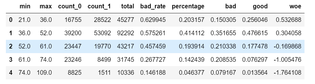
The process of selecting the best container is packaged into a function
def best_bin(DF,x,y,n=2,q=20,isshow=True):
"""
data:Data to be passed in
x:Column name to be boxed
y: Tag name corresponding to data
n:Number of boxes reserved
q:Number of boxes at the beginning
isshow:Whether to draw or not. The default is yes True
"""
DF = DF[[x,y]].copy() # Copy two columns with x and y
DF['qcut'],updown = pd.qcut(DF[x],retbins=True,q=q,duplicates='drop')
# Group aggregation calculates the number of 0 and 1 in the distribution box.
count_0 = DF[DF[y] == 0].groupby(by='qcut').count()[y]
count_1 = DF[DF[y] == 1].groupby(by='qcut').count()[y]
# Pack the upper and lower limits of each box, the number of 0 and the number of 1 together
num_bins = [*zip(updown,updown[1:],count_0,count_1)]
# print(num_bins)
# Make sure there are 0 and 1 in each box
for i in range(q):
if 0 in num_bins[0][2:]:
num_bins[0:2]=[(
num_bins[0][0]
,num_bins[1][1]
,num_bins[0][2]+num_bins[1][2]
,num_bins[1][3]+num_bins[1][3])]
"""If there is zero or empty in the first row, merge it with the next row,
At this time, we should also consider that the merged rows may not contain positive samples and negative samples
So we need to get back to this place if The position, judgment, that is, the cycle of adding the number of boxes,
One at a time continue,Go back and judge until there must be positive and negative samples in the row"""
continue
for i in range(len(num_bins)):
if 0 in num_bins[i][2:]:
num_bins[i-1:i+1]=[(
num_bins[i-1][0]
,num_bins[i][1]
,num_bins[i-1][2]+num_bins[i][2]
,num_bins[i-1][3]+num_bins[i][3])]
break
"""This is not to merge with the next row, because each row needs to be checked. The last row has no later row, so it is merged with the previous row, and the first row has been verified at the beginning"""
"""this break,Only in if It will be triggered only when the conditions are met
In other words, only when a merge occurs will it be interrupted for i in range(len(num_bins))This cycle
Why break the cycle? Because we are range(len(num_bins))Medium traversal
But after the merger, len(num_bins)Changes have taken place, but the cycle will not start again"""
else:
break
def get_woe(num_bins):
column = ['min','max','count_0','count_1']
num_bin = pd.DataFrame(num_bins,columns=column)
num_bin['total'] = num_bin.count_0 + num_bin.count_1
num_bin['bad_rate'] = num_bin.count_1/num_bin.total
num_bin['percentage'] = num_bin.total/num_bin.total.sum()
num_bin['bad'] = num_bin.count_0/num_bin.count_0.sum()
num_bin['good'] = num_bin.count_1/num_bin.count_1.sum()
num_bin['woe'] = np.log(num_bin['good']/num_bin['bad'])
return num_bin
def get_iv(num_bin):
    rate = num_bin['good'] - num_bin['bad']
    iv = np.sum(rate * num_bin.woe)
    return iv
# Calculate the maximum p value
iv_nums = []
axisx = []
while len(num_bins) > n: # Here n stands for the number of boxes to determine how many boxes to divide
pvs = []
for j in range(len(num_bins)-1):
pv = scipy.stats.chi2_contingency([num_bins[j][2:],num_bins[j+1][2:]])[1]
pvs.append(pv)
# print(pvs)
i = pvs.index(max(pvs))
# Observe the index where the maximum p value is located and determine that it is num_bins_ Generated from the first and second columns of data (starting from zero),
# Merge the first column and the second column. The beginning of the merged data is the beginning of the first column, and the end is the end of the second column. The amount of tree with label equal to 0,1 is the sum of the two columns
num_bins[i:i+2]= [(
num_bins[i][0],
num_bins[i+1][1],
num_bins[i][2]+num_bins[i+1][2],
num_bins[i][3]+num_bins[i+1][3])]
bins_df = pd.DataFrame(get_woe(num_bins))
axisx.append(len(num_bins))
iv_nums.append(get_iv(bins_df))
# print(bins_df)
# print(iv_nums)
if isshow:
plt.figure(figsize=(20,8),dpi=100)
plt.plot(axisx,iv_nums)
plt.xticks(axisx)
plt.show()
return Nonen_columns = model_data.columns
for i in n_columns[1:-1]:
print(i)
best_bin(model_data,i,'SeriousDlqin2yrs',n=2,q=20,isshow=True)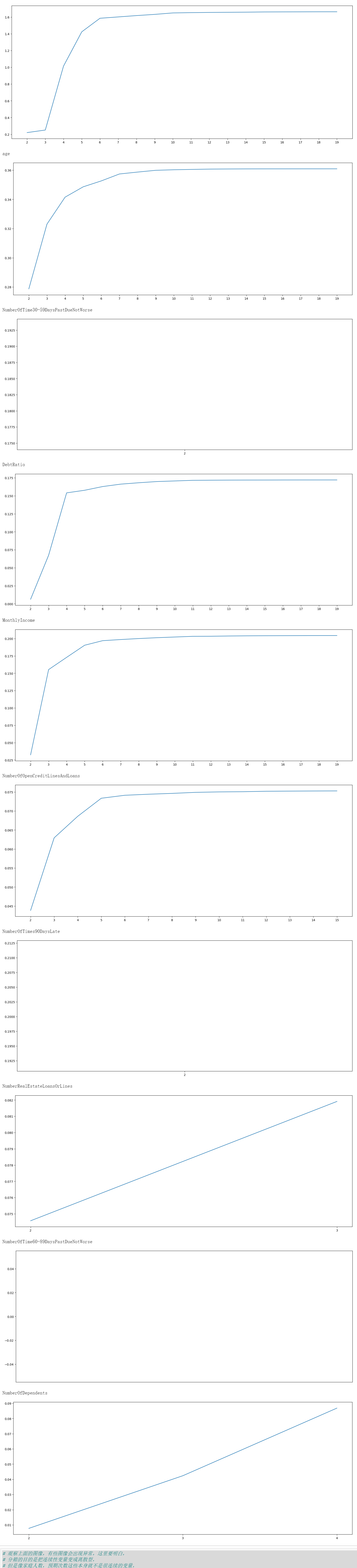
#Observe the above images. Some images will be abnormal. You should understand here,
#The purpose of dividing boxes is to change continuous variables into discrete ones,
#But variables such as family size and expected number of times are not very continuous in themselves,
#Therefore, this situation will occur when these characteristics are divided into boxes together with continuity variables
#At this time, you need to manually separate these results
auto_col_bins = {
    'RevolvingUtilizationOfUnsecuredLines':6,
    'age':5,
    'DebtRatio':4,
    'MonthlyIncome':4,
    'NumberOfOpenCreditLinesAndLoans':5
}

# Data requiring manual box splitting
hand_bins = {
    'NumberOfTime30-59DaysPastDueNotWorse':[0,1,213],
    'NumberOfTimes90DaysLate':[0,1,2,17],
    'NumberRealEstateLoansOrLines':[0,1,2,3,54],
    'NumberOfTime60-89DaysPastDueNotWorse':[0,1,2,11],
    'NumberOfDependents':[0,1,2,3,4,20]}

# Considering the actual situation, ensure the maximum coverage of the section, and use NP Inf replaces the maximum value with - NP Inf replaces the maximum (maximum and minimum)
hand_bins = {k:[-np.inf,*i[:-1],np.inf] for k,i in hand_bins.items()}
#Here I define a function of # optimal bin division result (it is found here that # when the bin division fails to meet the standard, the bins_df (i.e. bin division result) in the first function cannot be returned, and the data with normal bin division can be returned normally)
def best_bin_s(DF,x,y,n=2,q=20,isshow=True):
    """
    data:Data to be passed in
    x:Column name to be boxed
    y: Tag name corresponding to data
    n:Number of boxes reserved
    q:Number of boxes at the beginning
    isshow:Whether to draw or not. The default is yes True
    """
    DF = DF[[x,y]].copy() # Copy two columns with x and y

    DF['qcut'],updown = pd.qcut(DF[x],retbins=True,q=q,duplicates='drop')

    # Group aggregation calculates the number of 0 and 1 in the distribution box.
    count_0 = DF[DF[y] == 0].groupby(by='qcut').count()[y]
    count_1 = DF[DF[y] == 1].groupby(by='qcut').count()[y]
    # Pack the upper and lower limits of each box, the number of 0 and the number of 1 together
    num_bins = [*zip(updown,updown[1:],count_0,count_1)]

#     print(num_bins)

    # Make sure there are 0 and 1 in each box
    for i in range(q):
        if 0 in num_bins[0][2:]:
            num_bins[0:2]=[(
                    num_bins[0][0]
                    ,num_bins[1][1]
                    ,num_bins[0][2]+num_bins[1][2]
                    ,num_bins[1][3]+num_bins[1][3])]
            """If there is zero or empty in the first row, merge it with the next row,
            At this time, we should also consider that the merged rows may not contain positive samples and negative samples
            So we need to get back to this place if The position, judgment, that is, the cycle of adding the number of boxes,
            One at a time continue,Go back and judge until there must be positive and negative samples in the row"""
            continue
        for i in range(len(num_bins)):
            if 0 in num_bins[i][2:]:
                num_bins[i-1:i+1]=[(
                    num_bins[i-1][0]
                    ,num_bins[i][1]
                    ,num_bins[i-1][2]+num_bins[i][2]
                    ,num_bins[i-1][3]+num_bins[i][3])]
                break
                """This is not to merge with the next row, because each row needs to be checked. The last row has no later row, so it is merged with the previous row, and the first row has been verified at the beginning"""
                """this break,Only in if It will be triggered only when the conditions are met
                   In other words, only when a merge occurs will it be interrupted for i in range(len(num_bins))This cycle
                   Why break the cycle? Because we are range(len(num_bins))Medium traversal
                   But after the merger, len(num_bins)Changes have taken place, but the cycle will not start again"""
        else:
            break


    def get_woe(num_bins):

        column = ['min','max','count_0','count_1']

        num_bin = pd.DataFrame(num_bins,columns=column)

        num_bin['total'] = num_bin.count_0 + num_bin.count_1

        num_bin['bad_rate'] = num_bin.count_1/num_bin.total

        num_bin['percentage'] = num_bin.total/num_bin.total.sum()

        num_bin['bad'] = num_bin.count_0/num_bin.count_0.sum()

        num_bin['good'] = num_bin.count_1/num_bin.count_1.sum()

        num_bin['woe'] = np.log(num_bin['good']/num_bin['bad'])

        return num_bin

    def get_iv(num_bin):

        rate = num_bin['good'] - num_bin['bad']
        iv = np.sum(rate * num_bin.woe)
        return iv

    # Calculate the maximum p value

    iv_nums = []
    axisx = []

    while len(num_bins) > n: # Here n stands for the number of boxes to determine how many boxes to divide

        pvs = []

        for j in range(len(num_bins)-1):

            pv = scipy.stats.chi2_contingency([num_bins[j][2:],num_bins[j+1][2:]])[1]

            pvs.append(pv)

#             print(pvs)

        i = pvs.index(max(pvs))
        # Observe the index where the maximum p value is located and determine that it is num_bins_ Generated from the first and second columns of data (starting from zero),
        # Merge the first column and the second column. The beginning of the merged data is the beginning of the first column, and the end is the end of the second column. The amount of tree with label equal to 0,1 is the sum of the two columns
        num_bins[i:i+2]= [(
                        num_bins[i][0],
                        num_bins[i+1][1],
                        num_bins[i][2]+num_bins[i+1][2],
                        num_bins[i][3]+num_bins[i+1][3])]

        bins_df = pd.DataFrame(get_woe(num_bins))
        axisx.append(len(num_bins))
        iv_nums.append(get_iv(bins_df))
#         print(bins_df)
#         print(iv_nums)


    if isshow:
        plt.figure(figsize=(20,8),dpi=100)
        plt.plot(axisx,iv_nums)
        plt.xticks(axisx)
        plt.show()
    return bins_df
#Define the above function, pass in the characteristic data that can be automatically divided into boxes, let it return df with detailed information, and replace the minimum and maximum values with - NP inf,np. inf
bins_col = {}

for col in auto_col_bins:
    bins_df = best_bin_s(model_data,col,
                         'SeriousDlqin2yrs',
                         n=auto_col_bins[col],
                         q=20,isshow=False)

    bins_df = sorted(set(bins_df['min']).union(bins_df['max'])) # Returns the union of multiple sets

    bins_df[0],bins_df[-1] = -np.inf,np.inf

    bins_col[col] =bins_df

    bins_col.update(hand_bins)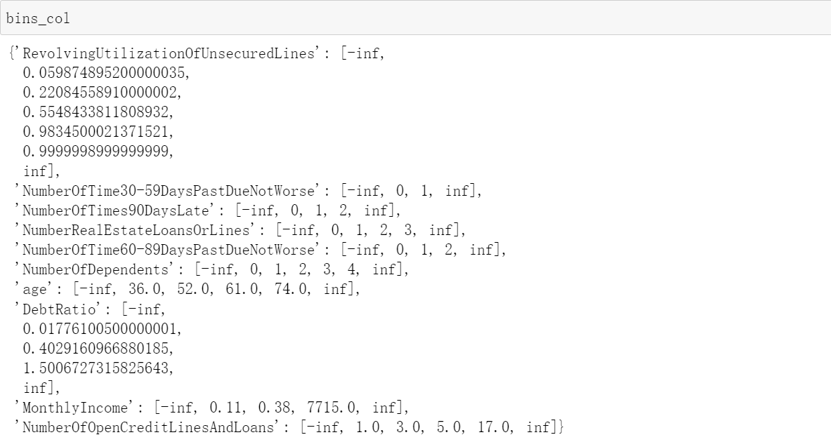
Calculate the WOE value of each box and map it to the data 
#When we use the function, the WOE value of the features that can be divided into boxes can be calculated automatically, but those that cannot be shared need to be processed manually
#Also replace the obtained WOE value (probability of non default without a box) with the original data model_ In data,
#Instead of using the original data, we want to use WOE to represent the difference of each box. What we want to obtain is the classification result of 'each box', that is, the classification result of each scoring item on the scoring card.
def new_get_woe(df,x,y,bins):
    df = df[[x,y]].copy()

    df['cut'] = pd.cut(df[x],bins)

    bins_df = df.groupby('cut')[y].value_counts().unstack()

    woe = bins_df['WOE'] = np.log((bins_df[0]/bins_df[0].sum()))/(bins_df[1]/bins_df[1].sum())

    return woe
woeall = {}
for col in bins_col:
woeall[col] = new_get_woe(model_data,col,'SeriousDlqin2yrs',bins_col[col])#Next, map all woe s to the original data
model_woe = pd.DataFrame(index=model_data.index)

# For all data--
for col in bins_col:

    model_woe[col] = pd.cut(model_data[col],bins_col[col]).map(woeall[col])

model_woe["SeriousDlqin2yrs"] = model_data["SeriousDlqin2yrs"]

#  This is the modeling data to be used (that is, the woe value of the box to which each data belongs)
model_woe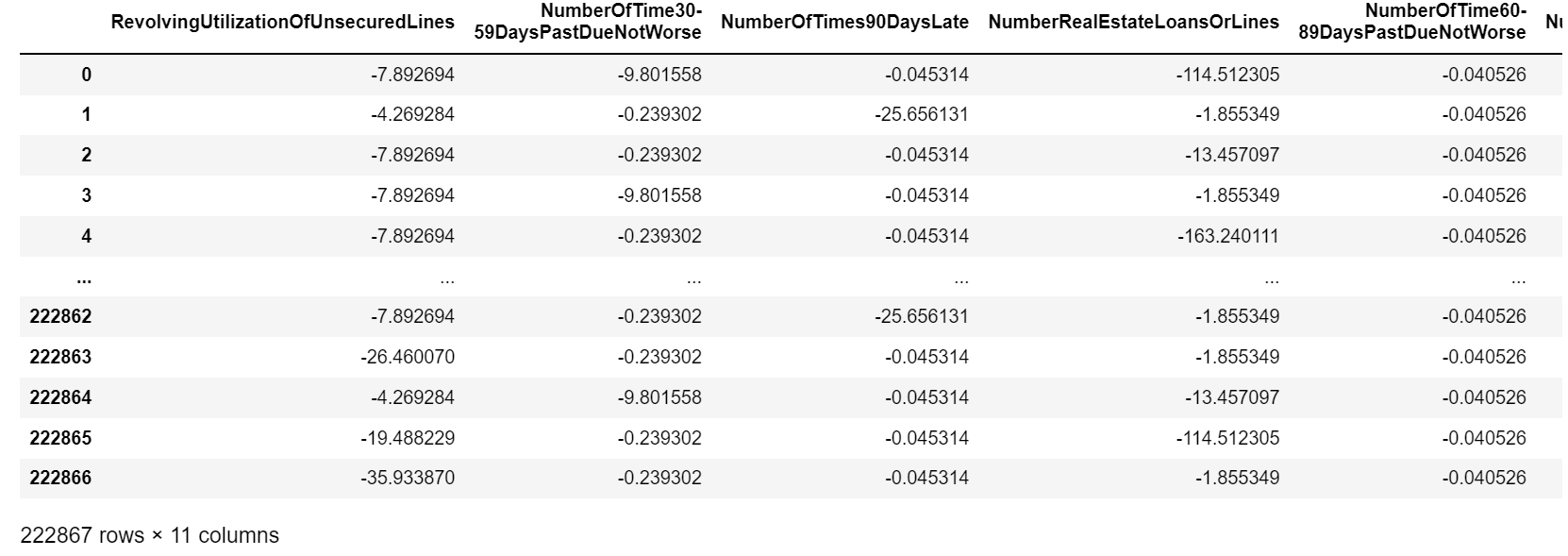
Modeling and model validation 
test_woe = pd.DataFrame(index=test_data.index)

# For all data--
for col in bins_col:

    test_woe[col] = pd.cut(test_data[col],bins_col[col]).map(woeall[col])


X = model_woe.iloc[:,:-1]
y = model_woe.iloc[:,-1]

test_x = test_woe.iloc[:,:-1]
test_y = test_woe.iloc[:,-1]
Machine learning:
lr = LR().fit(X,y)
lr.score(test_x,test_y)
Tuning:
c_1 = np.linspace(0.01,1,20)
c_2 = np.linspace(0.01,0.2,20)

import matplotlib.pyplot as plt
score = []
for i in c_2:
    lr = LR(solver='liblinear',C=i).fit(X,y)

    score.append(lr.score(test_x,test_y))


print(max(score),score.index(max(score)))
plt.figure(figsize=(20,8),dpi=80)

plt.plot(c_2,score)

plt.show()

lr.n_iter_ # View iterations

score = []
for i in [1,2,3,4,5,6]:
    lr = LR(solver='liblinear',C=0.01,max_iter=i).fit(X,y)
    score.append(lr.score(test_x,test_y))
plt.figure()
plt.plot([1,2,3,4,5,6],score)
plt.show()

# Get the optimal model
lr = LR(solver='liblinear',C=0.01,max_iter=i).fit(X,y)
lr.score(test_x,test_y)
# roc curve import scikitplot as skplt #%%cmd #pip install scikit-plot vali_proba_df = pd.DataFrame(lr.predict_proba(test_x)) skplt.metrics.plot_roc(test_y, vali_proba_df,plot_micro=False,figsize=(6,6),plot_macro=False)
Make score card:
#After modeling, we use accuracy and ROC curve to verify the prediction ability of the model. Next, let's talk about the transformation from logistic regression to standard scorecard. review
#The score in the scorecard is calculated by the following formula:
B = 20/np.log(2)
A = 600 + B*np.log(1/60)
B,A

# Calculation basis score
base_score = A - B*lr.intercept_ # intercept_  intercept
base_score

with open('./Data/ScoreData.csv','w')as f:
    f.write('base_score,{}\n'.format(base_score))

for i,col in enumerate(X.columns):
    score = woeall[col] * (-B*lr.coef_[0][i])
    score.name = "Score"
    score.index.name = col
    score.to_csv('./Data/ScoreData.csv',header=True,mode='a')
over!