Introduction: In this paper, the time-frequency correlation distribution algorithm is used to analyze the active sonar detection sound signal from a submarine in video, but it is still unable to get the result of the frequency change that the submarine and its supervisor hear. The exact reason is not yet understood.
Keywords: Submarine, Sonar, Joint Time-Frequency Distribution
_01 Signal Source
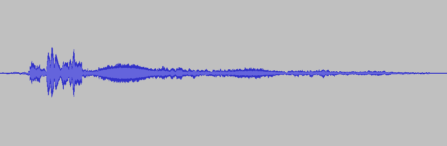
_This sound comes from the watermelon video Why are helicopters enemies of submarines? How does it counter-submarine? The sonar audio from the active submarine given by the oil tube is given in this paper, and the thermographic distribution of the joint distribution of the following spectrum is also given.
The download link for this audio signal on the CSDN is given below:
- Active submarine sonar audio signal : https://download.csdn.net/download/zhuoqingjoking97298/79515528
_Then, the next question remains, how exactly is the heat map corresponding to the above joint distribution of sound and video produced?
_02 analysis signal
_Next, the uploaded audio signal is analyzed in AI Studio.
2.1 Read in display signal
_First upload the stored audio files to AI Studio. In order to read the MP3 data files using the pydub module, the pydub software module needs to be pre-installed.
2.1.1 Read display code
import sys,os,math,time
import matplotlib.pyplot as plt
from numpy import *
from scipy.io import wavfile

submp3 = '/home/aistudio/data/submarine.mp3'
subwav = '/home/aistudio/data/submarine.wav'

from pydub import AudioSegment
sound = AudioSegment.from_file(file=submp3)
left =  sound.split_to_mono()[0]
sample_rate = sound.frame_rate
sig = frombuffer(left._data, int16)

print("sample_rate: {}".format(sample_rate), "len(sig): {}".format(len(sig)))

plt.clf()
plt.figure(figsize=(10,6))
plt.plot(sig)
plt.xlabel("n")
plt.ylabel("wave")
plt.grid(True)
plt.tight_layout()
plt.savefig('/home/aistudio/stdout.jpg')
plt.show()
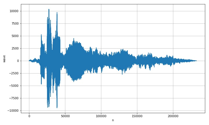
sample_rate: 44100
len(sig): 232448
2.2 Joint Time-Frequency Analysis
from scipy import signal

startid = 2
endid = 350
f,t,Sxx = signal.spectrogram(sig, fs=sample_rate,
                             nperseg=2048, noverlap=1024, nfft=8192)

thresh = 50
Sxx[where(Sxx > thresh)] = thresh

plt.clf()
plt.figure(figsize=(10,6))
plt.pcolormesh(t, f[startid:endid], Sxx[startid:endid, :])
plt.xlabel('Time(s)')
plt.ylabel('Frequency(Hz)')
plt.grid(True)
plt.tight_layout()
plt.savefig('/home/aistudio/stdout.jpg')
plt.show()
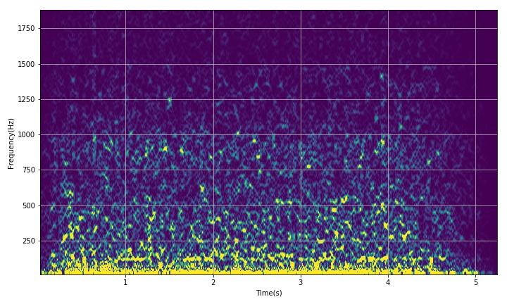
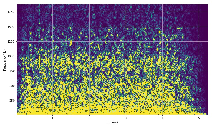
2.2.1 Analysis results
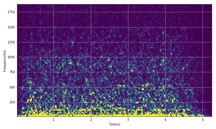
_Use SciPy above. The spectrogram in the signal gives the result of the video joint distribution of the signal, so it is always impossible to show the spectrum structure in the original video given in the motion diagram above.
_In addition, in terms of actual hearing, it is true that you can hear some frequency changes. However, this change cannot be seen from the result of the joint distribution of the resulting videos. It now seems most likely that there is a problem with the results given above.
_Analysis and Summary_
_This paper uses the time-frequency correlation distribution algorithm to analyze the active sonar detection sound signal from a submarine in the video, but it is still unable to get the result of the frequency change with the supervisor. The exact reason is not yet understood.
3.1 Processing Code
#!/usr/local/bin/python
# -*- coding: gbk -*-
#============================================================
# TEST1.PY                     -- by Dr. ZhuoQing 2022-02-07
#
# Note:
#============================================================

from headm import *                 # =
from scipy.io import wavfile


submp3 = '/home/aistudio/data/submarine.mp3'
subwav = '/home/aistudio/data/submarine.wav'

#sample_rate,sig = wavfile.read(subwav)
#printt(sample_rate:, len(sig):)

from pydub import AudioSegment
sound = AudioSegment.from_file(file=submp3)
left =  sound.split_to_mono()[0]
sample_rate = sound.frame_rate
sig = frombuffer(left._data, int16)

printt(sample_rate:, len(sig):)

#------------------------------------------------------------


plt.clf()
plt.figure(figsize=(10,6))
plt.plot(sig)
plt.xlabel("n")
plt.ylabel("wave")
plt.grid(True)
plt.tight_layout()
plt.savefig('/home/aistudio/stdout.jpg')
plt.show()

#------------------------------------------------------------
from scipy import signal


startid = 5
endid = 350
f,t,Sxx = signal.spectrogram(sig, fs=sample_rate,
                             nperseg=4096, noverlap=4000, nfft=8192)

thresh = 20
Sxx[where(Sxx > thresh)] = thresh

plt.clf()
plt.figure(figsize=(10,6))
plt.pcolormesh(t, f[startid:endid], Sxx[startid:endid, :])
plt.xlabel('Time(s)')
plt.ylabel('Frequency(Hz)')
plt.grid(True)
plt.tight_layout()
plt.savefig('/home/aistudio/stdout.jpg')
plt.show()


#------------------------------------------------------------
#        END OF FILE : TEST1.PY
#============================================================
Links to related literature:
- Why are helicopters enemies of submarines? How does it counter-submarine?
- Active Submarine Sonar Audio Signal. - spark Document Class Resource-CSDN Library
Related chart links: