Plans completed this week
- Read the pathological tissue segmentation paper full revolutionary multi class multiple instance learning
- Learned the operation of cutting large pathological images and corresponding labels into patch es
- Learned the DeepLabv3 + model
catalogue
Statistics on the proportion of each category
Thesis reading
Full convolutional multi class multiple instance learning
ABSTRACT (ABSTRACT)
Multi instance learning (MIL) can reduce the need for expensive annotation in tasks such as semantic segmentation by weakening the required degree of supervision. We propose a new mil formula for multi class semantic segmentation learning based on complete convolution network. In this case, we try to learn idiom meaning segmentation model from weak image level tags. The model is trained end-to-end to be represented by joint optimization, and the ambiguity of pixel image label assignment is eliminated. Full convolution training accepts input of any size, does not require object recommendation preprocessing, and provides pixel level loss map to select potential instances. Our multi class MIL Loss takes advantage of the further supervision provided by images with multiple tags. We evaluated this method through preliminary experiments on Pascal VOC segmentation challenge.
1 INTRODUCTION
In this work, we propose a new multi example learning (MIL) framework with complete convolution network (FCN). Its task is to learn pixel level semantic segmentation from weak image level labels that only represent the existence or absence of objects. Tagged objects that are not centered or images that contain multiple objects can make the problem more difficult. The main work of this paper is to drive the joint learning of ConvNet representation and pixel classifier through multi instance learning. Complete convolution training learns the model end-to-end at each pixel. In order to learn the segmentation model from the image tag, we project each image into a bag pixel level instance, and define the pixel level and multi class adaptive loss of mil.
We studied the following ideas and conducted preliminary experiments:
- We perform MIL in combination with end-to-end representation learning in a fully convolutional network. This eliminates the need to instantiate the instance tag hypothesis. FCN learning and reasoning can process images of different sizes without deformation or target recommendation preprocessing. This makes training simple and fast.
- We propose a multi class pixel level loss inspired by binary MIL scenes. This attempts to maximize the classification score based on each pixel instance, while using inter class competition to narrow the range of instance assumptions.
- Our goal is to weakly supervised image segmentation, which has not been studied. We believe that pixel level consistency cues are helpful to eliminate the ambiguity of objects. In this way, the weak segmentation can contain more image structures than the bounding box.
2 full convolutional MIL
For weakly supervised MIL learning, FCN allows effective selection of training examples. FCN predicts the output map of all pixels and has the corresponding loss map of all pixels. The loss graph may be masked, reweighted, or otherwise operated to select and select instances for calculating losses and back propagation for learning.
We use a VGG 16 layer network and convert it to a fully convoluted form as suggested by Long et al. Semantic segmentation is performed by replacing the fully connected layer with the corresponding convolution. The network is fine tuned according to the pre trained ILSVRC classifier weight, that is, pre trained to predict image level labels. Then, we experiment without initializing the last layer of weight (i.e. classifier layer). These initializations act as baselines without MIL tuning (rows 1 and 2 in the table). Without image level pre training, the model will quickly converge to all backgrounds. Semantic segmentation requires a background class, but the classification task does not have a background class; We simply initialize the background classifier weight to zero.
3 MULTI-CLASS MIL LOSS
We define the multi category MIL loss as the multi category loss calculated at the maximum predicted value. The output map generated by FCN is realized, that is, for images of any size, FCN outputs the heat map of each category (including background) of corresponding size. We determine the maximum score pixel in the rough heat map of the class existing in the image and background. Then, the loss is calculated only on these coarse points and back propagated through the network.

 Represents the input image,
 Is the label corresponding to the image,
 Yes
Yes The label is in
 Heat map of position output
For a picture, input it into the segmentation network to obtain a (N,H,W) segmentation map. The prediction of the picture for each class is stored as a feature map.
The Loss takes the maximum value on each map, and the calculation formula is shown in the figure above. Then, the maximum score is constrained to limit the existence of the category in the picture. If the label of the picture indicates an existing class, the score is close to 1, and if it does not exist, it is close to 0.
To put it simply, the maximum value on feature maps is limited to 1 to make the predicted value of the class that should exist large, and the maximum value is limited to 0 to make the predicted value of the class that should not exist small.
4 EXPERIMENTS
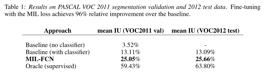
All results are from Pascal VOC segmentation challenge competition. The results are as follows:
5 DISCUSSION
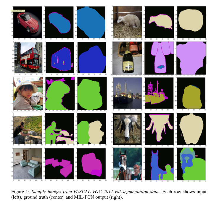
In this paper, a joint multi instance representation learning model of multi class pixel level loss inspired by two classes of MIL is proposed. The model learns end-to-end as a complete convolution network for weakly supervised semantic segmentation tasks. It eliminates the need for any type of instance or hypothesis mechanism, and the reasoning speed is fast (≈ 1 / 5 second). These results are encouraging and can be further improved. At present, our coarse-grained output is only linear interpolation. If we use conditional random field regularization or super-pixel projection, we can refine the prediction results.
SWI slice code implementation
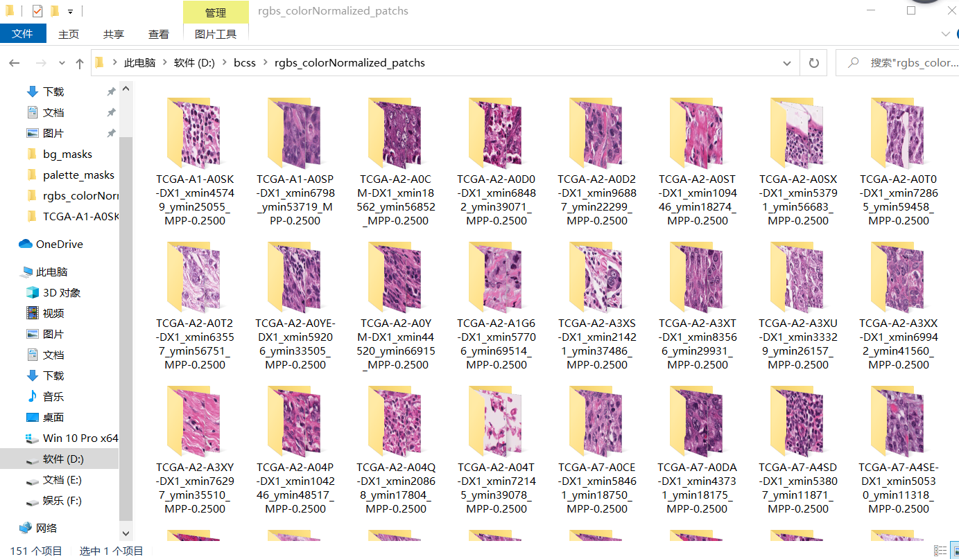
Because pathological images are large pixels, in order to reuse the limited data, large pathological images are generally sliced. There are 151 pathological images with mask in the data set sent by the teacher.
For each large pathological image before segmentation, 3394 * 2467 pixels and its corresponding mask (color with dye board)


Segmented patch, 256 * 256 pixels per patch

Palette tools
import os
import glob
import logging
import time
from shutil import copyfile
from multiprocessing import Pool, Value, Lock
from PIL import Image
import numpy as np
import torch


LABEL_PATH = 'D:\\bcss\\masks\\'  # The fifth path is the place where the label mask is placed, which are the black pictures
PALLET_LABEL_PATH = "D:\\bcss\\palette_masks\\"

import cv2
import os
import numpy as np
from PIL import Image

import cv2
import os
import numpy as np
from PIL import Image


def colorful(img, save_path):

    '''
    img:Pictures to be colored
    save_path:Storage path
    '''

    # print(np.unique(img))
    img = Image.fromarray(img)  # Convert the image from the data format of numpy to the image format in PIL
    palette = []
    for i in range(256):
        palette.extend((i, i, i))
    palette[:3 * 22] = np.array([[0, 0, 0],  # outside_roi 	 0 black doesn't care
                                 [128, 0, 0],  # tumor	1 Maroon tumor # follow
                                 [0, 128, 0],  # stroma	2 Green matrix # follow
                                 [128, 128, 0],  # lymphocytic_infiltrate 3 Light brown infiltration # follow
                                 [0, 0, 128],  # necrosis_or_debris	4 Tibetan green necrosis # follow
                                 [128, 0, 128],  # glandular_secretions 	 5 Purple gland secretion
                                 [0, 128, 128],  # blood 6 blue green blood
                                 [128, 128, 128],  # exclude 7 grey exclusion
                                 [64, 0, 0],  # metaplasia_NOS 8 metaplasia is colorless and its name is a little dark reddish brown
                                 [192, 0, 0],  # fat 9 fat is colorless and a little light red
                                 [64, 128, 0],  # plasma_cells 10 plasma cells are colorless and a little green
                                 [192, 128, 0],  # other_immune_infiltrate 	 Other immune infiltrates are colorless and a little light orange
                                 [64, 0, 128],  # mucoid_material 12 myxoid substance is colorless and its name is a little blue purple
                                 [192, 0, 128],  # normal_acinus_or_duct 13 Normal acini or ducts are colorless and named dark pink  # follow
                                 [64, 128, 128],  # lymphatics 	 The name of lymphatic system is colorless and a little blue-green
                                 [192, 128, 128],  # undetermined 	 15 the undetermined colorless name is a little light powder
                                 [0, 64, 0],  # nerve 	 16 nerve colorless dark green
                                 [128, 64, 0],  # skin_adnexa 	 17. The name of the skin accessory is colorless and a little brown
                                 [0, 192, 0],  # blood_vessel 	 18 blood vessels colorless name light green
                                 [128, 192, 0],  # angioinvasion 	 19 vascular invasion colorless name a little light dark green
                                 [0, 64, 128],  # dcis 	 20 breast carcinoma in situ colorless name a little light dark blue
                                 [224, 128, 64],  # other 	 Other colorless names are a little light orange
                                 ], dtype='uint8').flatten()

    img.putpalette(palette)
    print(np.unique(img))
    img.save(save_path)


def run():
    print("===================================================")
    # Path of black graph
    wsi_mask_paths = glob.glob(os.path.join(LABEL_PATH, '*.png'))
    num = 0
    for wsi_mask_path in wsi_mask_paths:
        # obtain the wsi path

        name = wsi_mask_path.split('\\')[-1]
        pid = name[:-4]
        print(name)
        print('pid', pid)
        num += 1
        print("Processing section{}Zhang mask image pid = {}".format(num , pid))
        print("num = ",num)


        # Open Black map
        img_label_mask = Image.open(wsi_mask_path)
        img_label_mask = np.array(img_label_mask)
        colorful(img_label_mask, os.path.join(PALLET_LABEL_PATH, str(pid))+ '.png')


if __name__ == '__main__':
    run()
Cut patch code
import os
import glob
import logging
import time
from shutil import copyfile
from multiprocessing import Pool, Value, Lock
from PIL import Image
import numpy as np
import torch
from convert_palette_imgs import colorful
def run2():
# Put the cut label patch on the path
if not os.path.exists(TRAIN_PATCH_PATH):
os.mkdir(TRAIN_PATCH_PATH)
# TRAIN_PATH: the path is to place the original image and find all the original images through the original image path
wsi_paths = glob.glob(os.path.join(TRAIN_PATH, '*.png'))
# Path of black graph
wsi_mask_paths = glob.glob(os.path.join(MASK_PATH, '*.png'))
# Path of color map
pallet_mask_paths = glob.glob(os.path.join(PALETTE_MASK_PATH, '*.png'))
cur_patch_cords = []
patch_name_list = []
mask_patch_name_list = []
pallet_mask_patch_name_list = []
train_data_lib = {}
# wsi_path the path of each original image
num = 0
for wsi_path,wsi_mask_path,pallet_mask_path in zip(wsi_paths,wsi_mask_paths,pallet_mask_paths):
# obtain the wsi path
name = wsi_path.split('\\')[-1]
pid = name[:-4]
print(name)
print('pid',pid)
num += 1
print("Processing section{}Pathological images pid = {}".format(num , pid))
print("num = ",num)
# gen the folder as the pathological number
# TRAIN_PATCH_PATH: put the cut label patch in the path
ID_PATH = TRAIN_PATCH_PATH
print(ID_PATH)
# # Open Black map
# img_label_mask = Image.open(wsi_mask_path)
# # img_label_mask.mode = L
# # print("img_label_mask.mode = ",img_label_mask.mode)
# img_label_mask = np.array(img_label_mask)
# Open color map
img_pallet_label_mask = Image.open(pallet_mask_path)
img_pallet_label_mask = np.array(img_pallet_label_mask)
# open the slide image
img = Image.open(wsi_path)
# MASK_PATH:mask diagram
# img_mask = Image.open(MASK_PATH+pid+'_mask.png')
img_mask = Image.open(MASK_PATH+pid+'.png')
width,height = img.size
print(width)
img = np.array(img)
img_mask = np.array(img_mask)
# gen the coordinates (x,y)
dd1 = []
dd2 = []
for i in range(0, width - patch_size, 128):
dd1.append(i)
for j in range(0, height - patch_size, 128):
dd2.append(j)
print("dd1 = ", dd1)
print("dd2 = ", dd2)
print("len(dd1) = ",len(dd1)," ---- "," len(dd2) = ",len(dd2)," ----- ","dd1*dd2 = ",len(dd1) * len(dd2))
# if width % patch_size / patch_size > 0.5:
# dd1.append(width - patch_size)
#
# if height % patch_size / patch_size > 0.5:
# dd2.append(height - patch_size)
# gen the patches as the coordinates and save them
for ii in range(len(dd1)):
for jj in range(len(dd2)):
# s = 0.6 * 256 * 256 * 255
# if np.sum(img_mask[int(dd1[ii]):int(dd1[ii])+patch_size, int(dd2[jj]):int(dd2[jj])+patch_size]) > s:
wsi_pallet_mask_patch = img_pallet_label_mask[int(dd1[ii]):int(dd1[ii]) + patch_size, int(dd2[jj]):int(dd2[jj]) + patch_size]
# wsi_mask_patch = img_label_mask[int(dd1[ii]):int(dd1[ii]) + patch_size, int(dd2[jj]):int(dd2[jj]) + patch_size]
img_patch = img[int(dd1[ii]):int(dd1[ii]) + patch_size, int(dd2[jj]):int(dd2[jj]) + patch_size]
img_mask_patch = img_mask[int(dd1[ii]):int(dd1[ii])+patch_size, int(dd2[jj]):int(dd2[jj])+patch_size]
# print(os.path.join(ID_PATH, str(pid) + '_' + str(dd1[ii]) + '_' + str(dd2[jj]) + '.png'))
if img_patch.shape[0] == 256 & img_patch.shape[1] == 256:
# print("img_patch.shape = ",img_patch.shape)
wsi_pallet_mask_patch = Image.fromarray(wsi_pallet_mask_patch)
# wsi_mask_patch = Image.fromarray(wsi_mask_patch)
img_patch=Image.fromarray(img_patch)
img_mask_patch = Image.fromarray(img_mask_patch)
if not os.path.exists(os.path.join(PALETTE_MASK_PATCH_PATH, str(pid))):
os.mkdir(os.path.join(PALETTE_MASK_PATCH_PATH, str(pid)))
colorful(np.array(wsi_pallet_mask_patch), os.path.join(PALETTE_MASK_PATCH_PATH, str(pid) +'\\'+ str(pid)+'_' + str(dd1[ii]) + '_'+ str(dd2[jj]) + '.png'))
# wsi_pallet_mask_patch.save(os.path.join(PALLET_MASK_PATCH_PATH, str(pid) +'\\'+ str(pid)+'_' + str(dd1[ii]) + '_'+ str(dd2[jj]) + '.png'))
pallet_mask_patch_name_list.append(os.path.join(PALETTE_MASK_PATCH_PATH, str(pid) + '_' + str(dd1[ii]) + '_' + str(dd2[jj]) + '.png'))
# if not os.path.exists(os.path.join(LABEL_PATCH_PATH, str(pid))):
# os.mkdir(os.path.join(LABEL_PATCH_PATH, str(pid)))
# wsi_mask_patch.save(os.path.join(LABEL_PATCH_PATH, str(pid) +'\\'+ str(pid)+'_' + str(dd1[ii]) + '_'+ str(dd2[jj]) + '.png'))
# mask_patch_name_list.append(os.path.join(LABEL_PATCH_PATH, str(pid) + '_' + str(dd1[ii]) + '_' + str(dd2[jj]) + '.png'))
if not os.path.exists(os.path.join(ID_PATH, str(pid))):
os.mkdir(os.path.join(ID_PATH, str(pid)))
img_patch.save(os.path.join(ID_PATH, str(pid) +'\\'+ str(pid)+'_' + str(dd1[ii]) + '_' + str(dd2[jj]) + '.png'))
patch_name_list.append(os.path.join(ID_PATH, str(pid) + '_' + str(dd1[ii]) + '_' + str(dd2[jj]) + '.png'))
if not os.path.exists(os.path.join(MASK_PATCH_PATH, str(pid))):
os.mkdir(os.path.join(MASK_PATCH_PATH, str(pid)))
img_mask_patch.save(os.path.join(MASK_PATCH_PATH, str(pid) +'\\'+ str(pid)+ '_' + str(dd1[ii]) + '_'+ str(dd2[jj]) + '.png'))
cur_patch_cords.append(os.path.join(MASK_PATCH_PATH, str(pid) + '_' + str(dd1[ii]) + '_' + str(dd2[jj]) + '.png'))
train_data_lib['mask_patch_name_list'] = mask_patch_name_list
train_data_lib['mask_patch_name_list'] = mask_patch_name_list
train_data_lib['patch_name_list']=patch_name_list
train_data_lib['cur_patch_cords']=cur_patch_cords
torch.save(train_data_lib, 'D:\\bcss\logs\\train_data_lib.db')
def main():
run2()
# img=Image.open('F:\\Oral_HE_IHCregistered_TMA\\train_mask_patch\\1_B-2_real_A_mask_1024_512.png')
# img = np.array(img)
# print(np.sum(img))
if __name__ == '__main__':
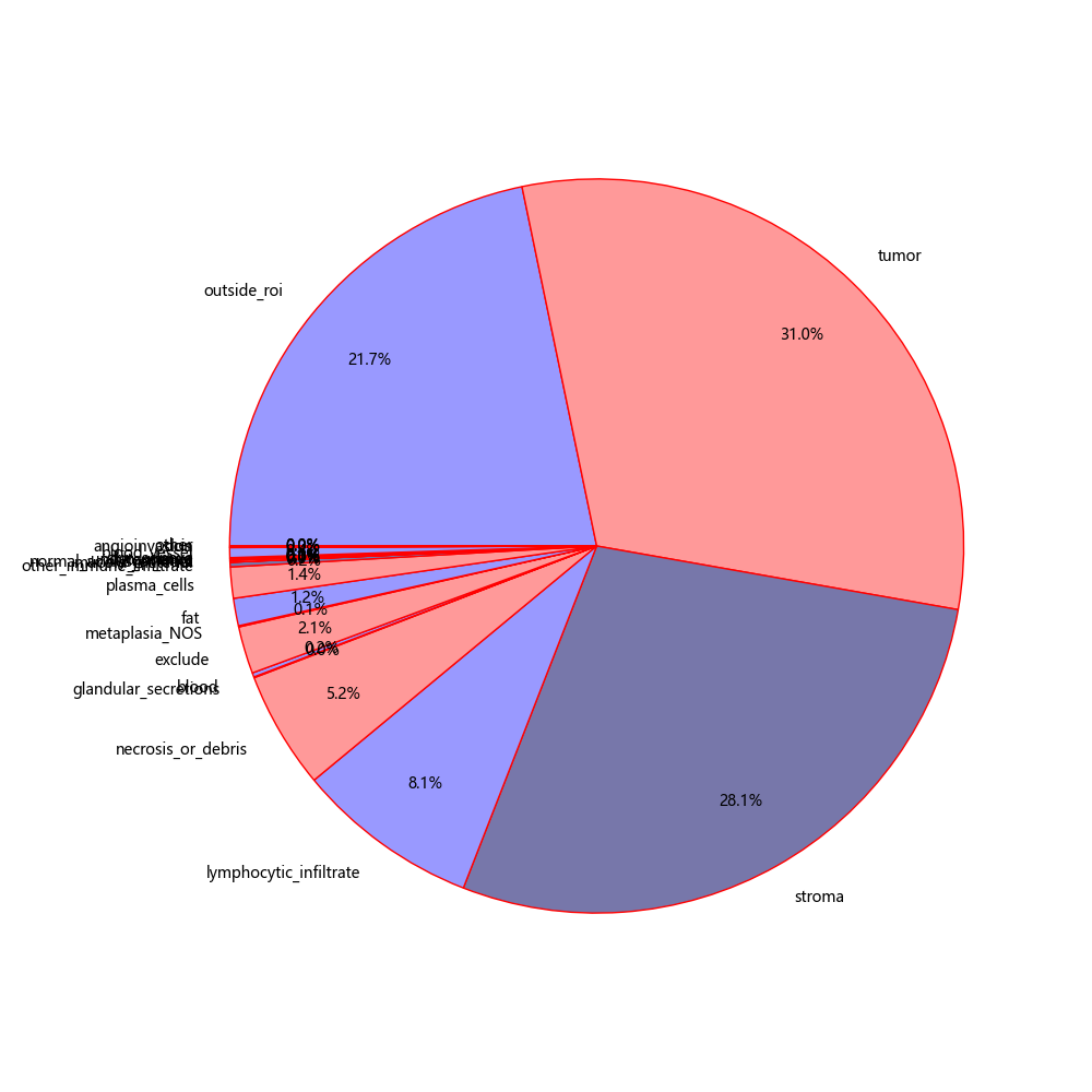
main()Statistics on the proportion of each category
Count the proportion of each pathological tissue, merge fewer tissue types, and re cut the patch
import json
import os
import glob
import logging
import time
from shutil import copyfile
from multiprocessing import Pool, Value, Lock
from PIL import Image
import numpy as np
import torch
import cv2
import matplotlib.pyplot as plt
"""

label	GT_code
outside_roi	0
tumor	1
stroma	2
lymphocytic_infiltrate	3
necrosis_or_debris	4
glandular_secretions	5
blood	6
exclude	7
metaplasia_NOS	8
fat	9
plasma_cells	10
other_immune_infiltrate	11
mucoid_material	12
normal_acinus_or_duct	13
lymphatics	14
undetermined	15
nerve	16
skin_adnexa	17
blood_vessel	18
angioinvasion	19
dcis	20
other	21

"""
LABEL_PATH = "D:\\bcss\\masks\\"
PALETTE_LABEL_PATH = "D:\\bcss\\palette_masks\\"

category_to_code = {"outside_roi":0,"tumor":1,"stroma":2,"lymphocytic_infiltrate":3,"necrosis_or_debris":4,
                            "glandular_secretions":5,"blood":6,"exclude":7,"metaplasia_NOS":8,"fat":9,"plasma_cells":10,
                            "other_immune_infiltrate":11,"mucoid_material":12,"normal_acinus_or_duct":13,"lymphatics":14,
                            "undetermined":15,"nerve":16,"skin_adnexa":17,"blood_vessel":18,"angioinvasion":19,"dcis":20,"other":21}
code_to_category = {0:"outside_roi",1:"tumor",2:"stroma",3:"lymphocytic_infiltrate",4:"necrosis_or_debris",
                    5:"glandular_secretions",6:"blood",7:"exclude",8:"metaplasia_NOS",9:"fat",10:"plasma_cells",
                    11:"other_immune_infiltrate",12:"mucoid_material",13:"normal_acinus_or_duct",14:"lymphatics",
                    15:"undetermined",16:"nerve",17:"skin_adnexa",18:"blood_vessel",19:"angioinvasion",20:"dcis",21:"other"}
all_imgs_category = {}
all_categories = {"outside_roi":0,"tumor":0,"stroma":0,"lymphocytic_infiltrate":0,"necrosis_or_debris":0,
                            "glandular_secretions":0,"blood":0,"exclude":0,"metaplasia_NOS":0,"fat":0,"plasma_cells":0,
                            "other_immune_infiltrate":0,"mucoid_material":0,"normal_acinus_or_duct":0,"lymphatics":0,
                            "undetermined":0,"nerve":0,"skin_adnexa":0,"blood_vessel":0,"angioinvasion":0,"dcis":0,"other":0}
def cal():
    print("=================== start cal ================================")
    # Path of black graph
    wsi_mask_paths = glob.glob(os.path.join(LABEL_PATH, '*.png'))
    wsi_palette_mask_paths = glob.glob(os.path.join(PALETTE_LABEL_PATH, '*.png'))
    print("len(wsi_mask_paths) = ",len(wsi_mask_paths))

    num = 0
    for wsi_mask_path,wsi_palette_mask_path in zip(wsi_mask_paths,wsi_palette_mask_paths):
        # obtain the wsi path
        print("wsi_palette_mask_path = ",wsi_palette_mask_path)
        name = wsi_mask_path.split('\\')[-1]
        print("name = ",name)
        wsi_mask_img = Image.open(wsi_mask_path)
        # img = plt.imread(wsi_palette_mask_path)
        # plt.title(wsi_palette_mask_path)
        # plt.imshow(img)
        # plt.show()
        # num += 1
        # if (num == 3):
        #     break
        wsi_mask_img_array = np.array(wsi_mask_img)
        print("wsi_mask_img_array.shape = ",wsi_mask_img_array.shape)
        h,w = wsi_mask_img_array.shape[0],wsi_mask_img_array.shape[1]
        # print("w = ",w," h = ",h)
        print("wsi_mask_img_array = ",wsi_mask_img_array)
        print("unique = ",np.unique(wsi_mask_img_array))
        print("="*50)
        print("=" * 50)
        # 2465-3392
        pid = name[:-4]

        # Count the number of occurrences of each category
        per_img_catogory = {"outside_roi":0,"tumor":0,"stroma":0,"lymphocytic_infiltrate":0,"necrosis_or_debris":0,
                            "glandular_secretions":0,"blood":0,"exclude":0,"metaplasia_NOS":0,"fat":0,"plasma_cells":0,
                            "other_immune_infiltrate":0,"mucoid_material":0,"normal_acinus_or_duct":0,"lymphatics":0,
                            "undetermined":0,"nerve":0,"skin_adnexa":0,"blood_vessel":0,"angioinvasion":0,"dcis":0,"other":0}

        print("per_img_catogory = ",per_img_catogory)
        for h_j in range(0,h - 1):
            for w_i in range(0, w - 1):
                pixel_mask = wsi_mask_img_array[h_j][w_i]
                for key,value in category_to_code.items():
                    if pixel_mask == value:
                        per_img_catogory[key] += 1
                        break
        # Add the statistics of each picture to the total statistics
        all_imgs_category[pid] = per_img_catogory


        print("per_img_catogory = ",per_img_catogory)
            #     print(pixel_mask,end=" ")
            #     print(str(h_j) + "-" + str(w_i))
            # print()

    # Print total statistics
    print("all_imgs_category = ",all_imgs_category)

    # Count the number of occurrences of each category in the total picture
    all_pixel = 0
    for key,value in all_imgs_category.items():
        # key is the name of each picture, and value is the number of pictures in each category
        for cate_name,cate_num in value.items():
            all_categories[cate_name] += cate_num
            all_pixel += cate_num
    all_category_count_percent = {}
    for key,value in all_categories.items():
        all_category_count_percent[key] = value / all_pixel

    # Write information to local json
    with open('./all_imgs_category.json', 'a', encoding='utf8') as fp:
        json.dump(all_imgs_category, fp, ensure_ascii=False)
    with open('./all_categories.json', 'a', encoding='utf8') as fp:
        json.dump(all_categories, fp, ensure_ascii=False)
    with open('./all_category_count_percent.json', 'a', encoding='utf8') as fp:
        json.dump(all_category_count_percent, fp, ensure_ascii=False)
    print("=================== end cal ================================")


def plot_categories(data_path):
    # Read the contents of the json file and return the dictionary format
    per_category_percent_names = []
    per_category_percent_values = []
    with open(data_path, 'r', encoding='utf8')as fp:
        json_data = json.load(fp)
        print('This is in the file json Data:', json_data)
        print('This is the data type of file data read:', type(json_data))
        for k,v in category_to_code.items():
            per_category_percent_name = k
            per_category_percent_value = json_data[k]

            per_category_percent_names.append(per_category_percent_name)
            per_category_percent_values.append(per_category_percent_value)
            # print(k + "-" + str(per_category_percent_value))
            # plt.figure(figsize=(12,8))
            # plt.plot()
    # Add decorated pie chart
    # explode = [0, 0.1, 0, ]  # Generate data to highlight B
    colors = ['#9999ff', '#ff9999', '#7777aa']  # Custom color

    # Treatment of Chinese garbled code and negative sign of coordinate axis
    plt.rcParams['font.sans-serif'] = ['Microsoft YaHei']
    plt.rcParams['axes.unicode_minus'] = False

    # Standardize the abscissa and ordinate axes to ensure that the pie chart is a positive circle, otherwise it is an ellipse
    plt.figure(figsize=(10, 10))
    plt.axes(aspect='equal')
    # Draw pie chart
    plt.pie(x=per_category_percent_values,  # Drawing data
            # explode=explode,  # Highlight B
            labels=per_category_percent_names,  # Add education level label
            colors=colors,  # Sets the custom fill color for the pie chart
            autopct='%.1f%%',  # Format the percentage with one decimal place
            pctdistance=0.8,  # Sets the distance between the percentage label and the center of the circle
            labeldistance=1.1,  # Sets the distance between the education level label and the center of the circle
            startangle=180,  # Sets the initial angle of the pie chart
            radius=2,  # Sets the radius of the pie chart
            counterclock=False,  # Whether it is counterclockwise, set it to clockwise here
            wedgeprops={'linewidth': 1, 'edgecolor': 'red'},  # Set the attribute values of the inner and outer boundaries of the pie chart
            textprops={'fontsize': 10, 'color': 'black'},  # Sets the attribute value of the text label
            )
    # plt.savefig('./categories_percents.png', dpi=100)  # It must be in PLT Before show()


    # Add diagram title
    # plt.title('proportion of each category ')
    # plt.savefig('./categories_percents.jpg', dpi=300)  # It must be in PLT Before show()
    fig = plt.gcf()
    fig.savefig('./categories_percents.png', format='png', transparent=True, dpi=20, pad_inches=0)
    # display graphics
    plt.show()
Work summary of this week
1. Learn to cut large pixel pathological images and corresponding labels into patch es, and make full use of the limited medical image data training network, because the pixel values of the labeled data of the image are not very different. If they are displayed directly, it is difficult for the naked eye to see what category they belong to. You can use the palette to dye different pixel values with different colors for easy observation
2. The weakly supervised paper full revolutionary multi class multiple instance learning, which I read, can achieve some effect by using image level label and pixel level segmentation with MIL Loss.