Supervised algorithm decision tree
1: Algorithm overview
Decision tree: includes classification tree / regression tree. Regression tree is rarely used, so classification tree is mainly introduced here
Algorithm flow: feature selection – > decision tree generation – > decision tree pruning
2: Feature selection
2.1 aroma entropy (information entropy)
Entropy represents the degree of information confusion. The more chaotic the information is, the higher the entropy is
Calculation formula of entropy:
E
n
t
r
o
p
y
(
m
)
=
−
∑
i
=
1
k
p
i
l
o
g
2
p
i
Entropy(m) = -\sum_{i=1}^{k}p^ilog_2p^i
Entropy(m)=−i=1∑kpilog2pi
When p=0, entropy = 0, because the certainty is 100%, there is no information confusion
#Calculation of information entropy
import numpy as np
p1 = 0.1
p2 = 0.9
s = -p1*np.log2(p1)-p2*np.log2(p2)
print(s)
Gini index
Φ ( p , 1 − p ) = 1 − ∑ i = 1 m p i 2 \Phi(p,1-p) = 1-\sum_{i=1}^{m}p_i^2 Φ(p,1−p)=1−i=1∑mpi2
Classification error
Φ ( p , 1 − p ) = 1 − m a x ( p , 1 − p ) \Phi(p,1-p) = 1-max(p,1-p) Φ(p,1−p)=1−max(p,1−p)
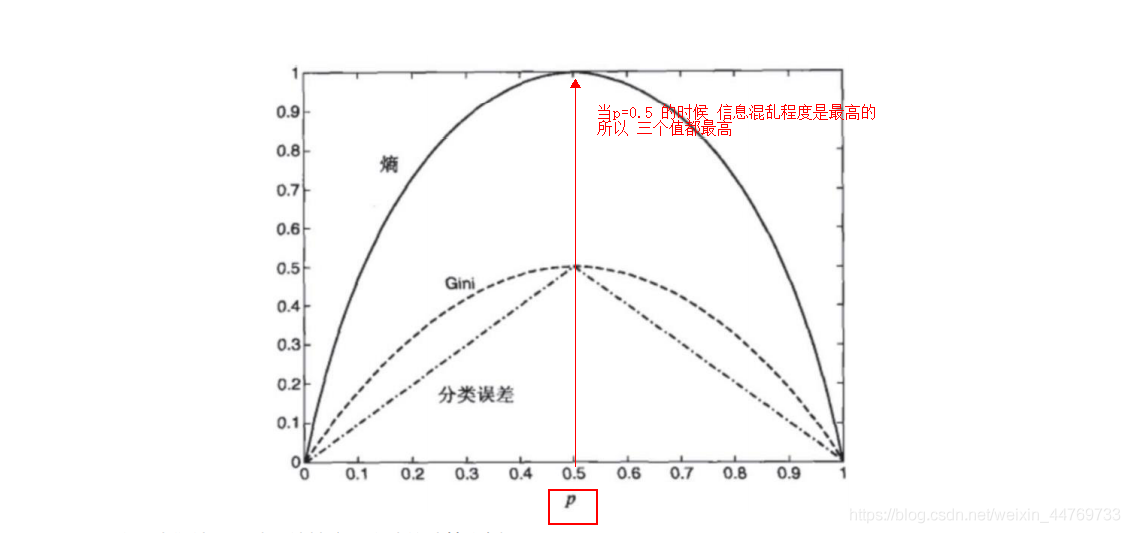
Code implementation of information entropy:
The entropy of all information is calculated here. Because it is calculated through the label column - gender, the entropy value is relatively high
#Code implementation of information entropy
#1. Data preparation
import pandas as pd
import numpy as np

data = pd.DataFrame(
    data={
        'Basketball':[0,1,1,1,0],
        'game':[1,0,0,1,1],
        'Gender':[0,1,1,0,0],
    }
)
print(data)

#Calculate the entropy of all data through the label column
def entropy(data):
    #Get number of rows
    rows = data.shape[0]
    #Get the gender column and find the number of each category
    sex_count = data.iloc[:,-1].value_counts()
    #Find the probability value
    p = sex_count / rows
    #Seeking entropy
    score = (-(p*np.log2(p))).sum()
    return score

entropy(data)  #0.9709505944546686
2.2 information gain
The greater the difference between the impure degree of the parent node (before partition) and the impure degree of the branch node (after partition), it means that the greater the "impure improvement" obtained by using attribute a for partition, the better the test condition effect.
Formula:
letter
interest
increase
benefit
=
I
(
father
section
spot
)
−
I
(
son
section
spot
)
father
section
spot
generation
surface
total
body
of
letter
interest
entropy
son
section
spot
generation
surface
finger
set
special
Dismantle
branch
of
after
of
letter
interest
entropy
Information gain = I (parent node) - I (child node) \ \ the parent node represents the overall information entropy \ \ the child node represents the information entropy after the specified special split
Information gain = I (parent node) − I (child node) the parent node represents the overall information entropy, and the child node represents the information entropy after the specified special split
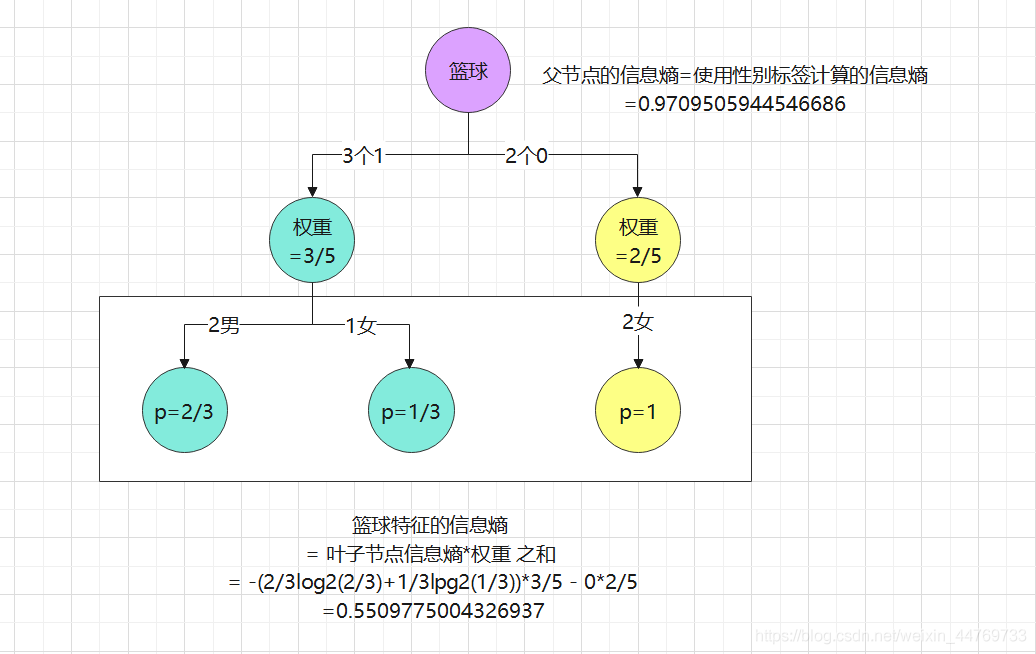
Case: calculate the information entropy of basketball
Data:
| Basketball | 0 | 1 | 1 | 1 | 0 |
|---|---|---|---|---|---|
| game | 0 | 0 | 0 | 0 | 1 |
| Gender | 0 | 1 | 1 | 0 | 0 |
Division: because the information entropy of basketball is calculated, basketball features are used for classification
Conclusion:
Information gain of basketball characteristics = 0.97 - 0.55 = 0.42
Similarly, calculate the information gain of the game = 0.97 - 0.8 = 0.17
Comparing the information gain of basketball and game, it shows that the information gain brought by the characteristics of basketball is greater. Therefore, on the premise of only these two characteristics, the characteristics of basketball should be used as the root node to disassemble the molecular node
2.3 dividing data sets
The maximum criterion for dividing data sets is to select the maximum information gain, that is, the direction in which the information decreases the fastest
Calculation of maximum information gain realized by code:
#Maximum information gain calculation
#1. Dataset
import pandas as pd
import numpy as np

data = pd.DataFrame(
    data={
        'Basketball':[0,1,1,1,0],
        'game':[0,0,0,0,1],
        'Gender':[0,1,1,0,0],
    }
)
print(data)

#2. Return the information entropy of the whole data set
def allEnt(data):
    #Number of rows
    n = data.shape[0]
    #Classification and probability of classification
    cnt = data.iloc[:,-1].value_counts()
    p = cnt/n
    #Information entropy
    ent = (-p*np.log2(p)).sum()
    return ent

#3. Loop through each column and label column to calculate information entropy
def preEnt(data):
    #First calculate the total entropy
    allent = allEnt(data)
    print('Total information entropy=',allent)
    #Total number of rows
    rows = data.shape[0]
    print('Total number of rows=',rows)
    #Define a variable to compare which feature has the highest information gain
    best = -1
    #The definition variable receives the column label because it changes every loop
    axis = 0


    for i in range(0,data.shape[1]-1): #Take one column of data at a time
        flags = data.iloc[:,i].value_counts().index #Get the type of each column
        print(flags)
        ent=0

        for j in flags: #Traverse the classification of each column, label the column by classification, and get the data set of each child node (this data set includes redundant features, but does not affect the calling function allEnt())
            childSet = data[data.iloc[:,i]==j] #Each sub data set
            #print(childSet)
            childEnt = allEnt(childSet) #Call the above method to find the information entropy of each subset
            #print(childEnt)
            ent += childEnt * (childSet.shape[0]/rows) #The information entropy of each child node is multiplied by the weight and then accumulated

        #Calculate information gain
        zy = allent - ent

        print('The first{}Information entropy of columns='.format(i),ent)
        print('The first{}Column information gain='.format(i),zy)

        #Determine which feature has the highest information gain
        if zy>= best:
            best = zy  #Assign the data with the highest information gain to best
            axis = i  #Assign the column label with the highest information gain to axis

    print('Highest information gain=',best)
    print('Column with the highest information gain=',axis)

    return best,axis

preEnt(data)  #Results: (0.4199730940219749, 0) represents the highest information gain = 0.42, and the data in column 0 produces the highest information gain
2.4 data set division by given column
In fact, the column with the highest information gain is calculated in the previous step, then the column label is obtained, and then the data set is divided
Objective: to prepare for further division
#Data is divided by the specified column and the classification of the specified column
#1. Dataset
import pandas as pd
import numpy as np

data = pd.DataFrame(
    data={
        'Basketball':[0,1,1,1,0],
        'game':[0,0,0,0,1],
        'Gender':[0,1,1,0,0],
    }
)
print(data)

#2. Divide the data set. According to the above, column 0 is the column with the highest information gain, so column 0 is used for division
def split(data,column,value):
    col = data.columns[column] #The name of the specified column was found
    childSet = data[data.iloc[:,column]==value] #Here is the data with value = value in the column
    childSet = childSet.drop(col,axis=1) #Delete the specified partitioned column

    return childSet

split(data,0,1) #
3: Decision tree algorithm
Algorithm principle: recursion
Algorithm classification: ID3 / C4 5 / C5. 0
The conditions for recursive constraints are:
- The program traverses all the attributes that divide the dataset
- All instances under each branch have the same classification
- The sample set contained in the current node is empty and cannot be divided
3.1 ID3
The core of ID3 algorithm is to apply information gain criterion to select features at each node of decision tree and construct decision tree recursively. The specific methods are:
- Starting from the root node, the information gain of all possible features is calculated for the node.
- The feature with the largest information gain is selected as the feature of the node, and the child nodes are established according to the different values of the feature.
- Then call the above methods on the child nodes to build a decision tree.
- Until the information gain of all features is very small or no features can be selected, finally a decision tree is obtained.
Disadvantages of ID3:
The limitation of ID3 algorithm mainly comes from the local optimization condition, that is, the calculation method of information gain. Its limitations mainly include the following points:
- The higher the branching degree (the more the classification level), the smaller the total information entropy of the child nodes, and ID3 is cut according to a certain column
The classification of some columns may not indicate the results well enough. In extreme cases, the ID is taken as the segmentation field, and each classification
The purity of is 100%, so this classification method is not effective. - Continuous variables cannot be processed directly. If ID3 is used to process continuous variables, the continuous variables need to be discretized first.
- It is sensitive to missing values. It is necessary to deal with the missing values in advance before using ID3.
- Without pruning, it is easy to lead to over fitting, that is, it performs well in the training set and poorly in the test set
3.2 C4.5
C4.5 is better than ID3 because it modifies the local optimization conditions
- ID3 takes the information gain as the feature of dividing the training data set, which is biased to select the feature with more values
- C4.5 this problem can be corrected by using information gain ratio.
- The gain rate criterion has a preference for attributes with a small number of values, so C4 5 the algorithm does not directly select the gain rate
Instead of the largest candidate partition attribute, a heuristic is used: first, find the genus whose information gain is higher than the average level from the candidate partition attributes
And then select the one with the highest gain rate.
Formula:
letter
interest
increase
benefit
rate
/
than
G
a
i
n
_
r
a
t
i
o
n
(
D
,
a
)
=
G
a
i
n
(
D
,
a
)
I
V
(
a
)
his
in
I
V
(
a
)
=
−
∑
v
=
1
V
∣
D
v
∣
∣
D
∣
l
o
g
2
∣
D
v
∣
∣
D
∣
I
V
(
a
)
call
call
by
genus
nature
/
special
sign
a
of
solid
have
value
,
V
generation
surface
special
sign
a
of
l
e
v
e
l
number
,
place
with
V
More
large
,
be
I
V
(
a
)
also
More
high
Gain / gain ratio\_ Ratio (D, a) = \ frac {gain (D, a)} {IV(a)} \ \ where IV(a) = - \ sum_ {v = 1} ^ {V} \ frac {| D} {| D} log2 \ frac {| D} {| D} \ \ IV(a) is called the intrinsic value of attribute / feature a, and V represents the level number of feature a, so the larger V, the higher IV(a)
Gain / gain ratio_ Ratio (D, a) = IV(a) gain (D, a), where IV(a) = − v=1 Σ V ∣ D ∣∣ Dv ∣ log2 ∣ D ∣∣ Dv ∣ IV(a) is called the intrinsic value of attribute / feature a, and V represents the level number of feature a, so the larger V, the higher IV(a)
Calculate information gain rate:
| Characteristic a | Characteristic b | label | |
|---|---|---|---|
| 0 | 0 | 1 | yes |
| 1 | 0 | 1 | yes |
| 2 | 0 | 0 | no |
| 3 | 1 | 1 | no |
| 4 | 1 | 1 | no |
According to the above data, calculate whether the information gain rate of feature a:
IV(a) = -3/5log2(3/5)-2/5log2(2/5) = 0.971
Total information entropy: ent_all = -2/5log2(2/5) -3/5log2(3/5)= 0.97
Information entropy of feature a: ent_a = -3/5*(2/3np.log2(2/3)+1/3np.log2(1/3))= 0.55
Information gain of feature a: Gain(D,a) = 0.97-0.55=0.42
Information increment ratio of feature a: Gain_ration(D,a) = 0.55/0.97 = 0.432
C4.5 how to deal with continuous variables:
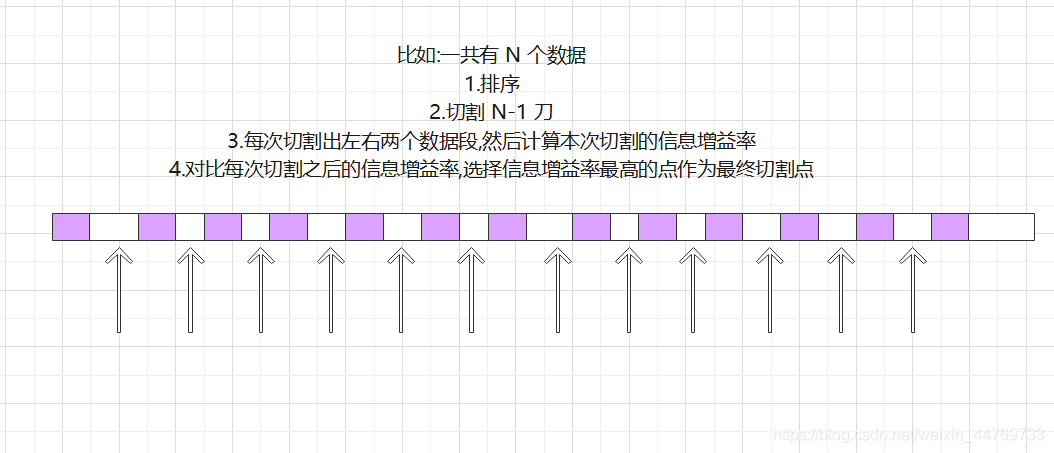
At C4 5, the processing means for continuous variables is also added. If the input characteristic field is a continuous variable, the algorithm will first
Sort the number of this column from small to large, and then select the middle number of two adjacent numbers as the candidate point of the segmented data set. If one is connected
If the continuation variable has N values, it is in C4 5 will generate N-1 alternative tangent points, and each tangent point represents a binary
Partition scheme of fork tree
4: Goodness of fit optimization (CART algorithm)
Judge whether it is over fit or under fit
prune
There is a unique solution to prevent over fitting of decision tree - pruning.
| pre-pruning | post-pruning | |
|---|---|---|
| Number of branches | Many branches are not expanded | Many branches are reserved |
| Fitting risk | The risk of over fitting is reduced, but the essence of greedy algorithm prohibits the expansion of subsequent branches, resulting in the risk of under fitting | Mr. Cheng becomes a decision tree and is assessed one by one from top to bottom. The risk of under fitting is small and the generalization ability is strong |
| Time cost | Low training and testing costs | Relatively small pre pruning |
Therefore, post pruning is commonly used
Pruning algorithm – CART algorithm:
- The splitting process is a binary recursive partitioning process
- The type of CART predictive variable x can be either continuous variable or subtype variable (if it is continuous variable, it needs to be transformed into dummy variable)
- The data shall be processed in its original form without discretization
- When used for numerical prediction, regression is not used, but the prediction is based on the average value of cases reaching leaf nodes
Splitting criterion of CART algorithm: binary splitting
Binary recursive partition: the condition holds to the left, and vice versa to the right
- For continuous variables: the condition is that the attribute is less than or equal to the optimal splitting point
- For category variables: the condition is that the attribute belongs to several classes
Advantages of binary splitting:
Compared with the slow speed of data fragmentation caused by multi-channel splitting, it allows repeated splitting on one attribute, that is, enough data can be generated on one attribute
The division of. The improvement of tree prediction performance brought by two-way splitting is enough to make up for the corresponding loss of tree readability.
For the predicted variables with different attributes, the y splitting criteria are different:
- Classification tree: Gini criterion. Similar to the previous information gain, Gini coefficient measures the impurity of a node.
- Regression tree: a common segmentation criterion is standard deviation reduction (SDR), similar to
- Least mean square error LS (least squares) criterion.
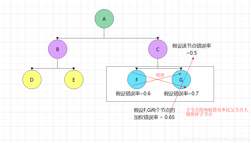
How to prune CART algorithm:
5: sklean generating decision tree
5.1 parameter criterion
| criterion two parameters | Entropy information entropy | gini Gini coefficient |
|---|---|---|
| - | It is more sensitive to impure, and the punishment for impure is the strongest | |
| - | The calculation is slow because it involves logarithmic operation | No logarithm, faster |
| - | The data with high latitude / noise is easy to be over fitted. If the model is under fitted, information entropy can be selected | Use of noisy data |
5.2 code implementation
#Implementing decision tree with sklean
#1. Import the required algorithm libraries and modules
import pandas as pd
import numpy as np
import matplotlib.pyplot as plt
%matplotlib inline

from sklearn import tree
from sklearn.datasets import load_wine
from sklearn.model_selection import train_test_split
plt.rcParams['font.sans-serif']=['Simhei']
plt.rcParams['axes.unicode_minus']=False

#2. Prepare data
wine = load_wine()
wine.data.shape
wine.target
wine_pd=pd.concat([pd.DataFrame(wine.data),pd.DataFrame(wine.target)],axis=1)
#wine.feature_name = ['alcohol', 'malic acid', 'ash', 'ash alkalinity', 'magnesium', 'total phenols',' flavonoids', 'non flavanophenols',' anthocyanins', 'color intensity', 'hue', 'od280/od315 diluted wine', 'proline']
wine.feature_names.append("result")
wine_pd.columns=wine.feature_names
wine_pd = wine_pd.rename(columns={
    'alcohol':'alcohol','malic_acid':'malic acid',
    'ash':'ash','alcalinity_of_ash':'Alkalinity of ash',
    'magnesium':'magnesium','total_phenols':'Total phenol',
    'flavanoids':'flavonoid','nonflavanoid_phenols':'Non flavane phenols',
    'proanthocyanins':'anthocyanin','color_intensity':'Color intensity',
    'hue':'tone','od280/od315_of_diluted_wines':'od280/od315 Diluted wine',
    'proline':'proline','result':'label'
})
print(wine_pd.head())

#3. Divide training set and test set
Xtrain,Xtest,Ytrain,Ytest = train_test_split(wine_pd.iloc[:,:-1],wine_pd.iloc[:,-1],test_size=0.3,random_state=420)

#4. Establish model
clf = tree.DecisionTreeClassifier(criterion='gini') #Use the gini parameter, which is also gini by default
#5. Training model
clf = clf.fit(Xtrain,Ytrain)
#6. Check accuracy
score = clf.score(Xtest,Ytest)
print(score) # 0.9444444444444444

#4. Draw trees
#Using the package: pip install graphviz, you also need to manually install plug-ins and set the system environment PATH (including bin directory and dot.exe under bin directory)
import graphviz
import matplotlib.pyplot as plt
feature_name = ['alcohol','malic acid','ash','Alkalinity of ash','magnesium','Total phenol','flavonoid','Non flavane phenols','anthocyanin','Color intensity','tone','od280/od315 Diluted wine','proline']
dot_data = tree.export_graphviz(clf, #Model
                                feature_names= feature_name, #Feature column name
                                class_names=["Gin","Shirley","Belmord"], #In fact, it corresponds to 0 / 1 / 2 of the label
                                filled=True, #Render color
                               )
graph = graphviz.Source(dot_data,filename='Decision tree PDF')
graph
export_graphviz generates the parameters of a decision tree in DOT format:
- feature_names: the name of each attribute
- class_names: the name of each dependent variable category
- Label: whether to display the label of impurity information. The default is "all", which can be "root" or "none"
- filled: whether to draw different colors for the main classification of each node. The default is False
- out_file: the name of the output dot file. The default is None, which means that the file is not output. It can be a user-defined name, such as "tree.dot"
- Rounded: the default is Ture, which means that the border of each node is rounded and Helvetica font is used
- More parameters: https://scikit-learn.org/stable/modules/generated/sklearn.tree.export_graphviz.html#sklearn.tree.export_graphviz
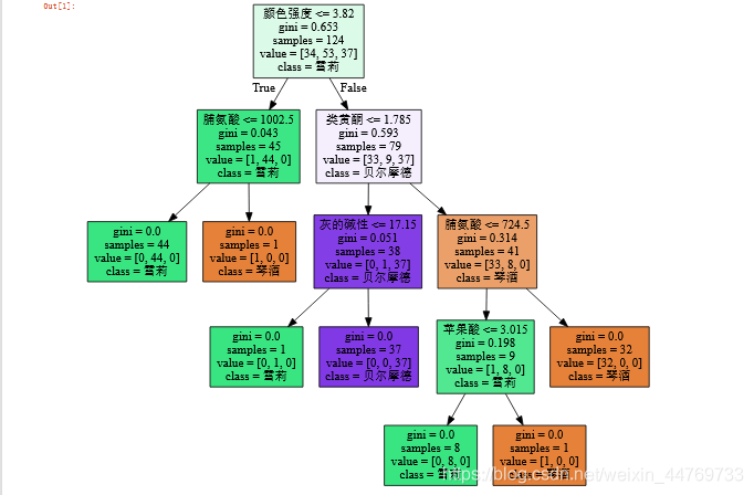
Preliminary appearance of decision tree:
6: Decision tree attribute
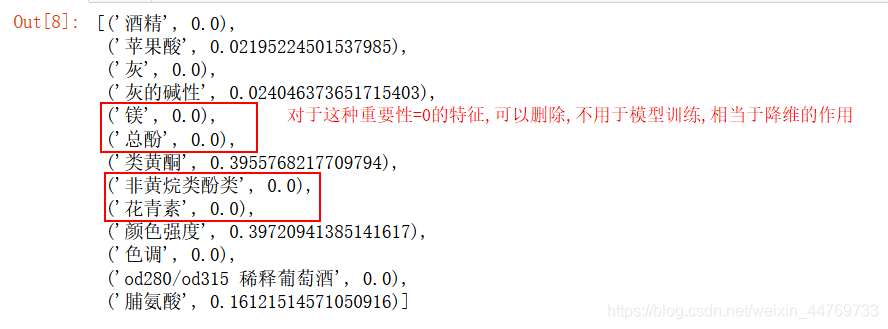
1.clf.feature_importances_
Show the importance of each feature
clf.feature_importances_

[*zip(feature_name,clf.feature_importances_)]
2.clf.apply
Returns the leaf index for each prediction sample
3.clf.tree_.node_count
Returns the number of nodes in the tree
4.clf.tree_.feature
Return the attribute index value corresponding to each node, - 2 indicates leaf node:
7: Prevent overfitting (pruning parameters)
7.1 parameter random_state random seed
Each time you set different random seeds, the resulting trees are different, so
tree.DecisionTreeClassifier(
    					criterion="entropy"
						,random_state=30   #This random seed can be changed at will
						,splitter="random"
						)
7.2 parameter splitter
splitter has two values:
1.splitter ='best'
Although the decision tree branches randomly, it will give priority to more important features for branching (the importance can be viewed through the attribute feature_imports_);
2.splitter ='random'
The possibility of over fitting can be reduced, but the post pruning is optimized by using the following pruning parameters
tree.DecisionTreeClassifier(
    					criterion="entropy"
						,random_state=30
						,splitter="random" #best / random
						)
7.3 pruning parameters:
7.3.1 max_depth limits the maximum depth of the tree
It is recommended to try from = 3 to see the fitting effect, and then decide whether to increase the set depth
7.3. 2 min_ samples_ At least the number of samples per node after leaf branch
If the value is too small, it will be over fitted and under fitted
It is recommended to start with = 5. If the sample size contained in the leaf node changes greatly, it is recommended to enter a floating-point number as a percentage of the sample size
7.3.3 min_samples_split each node must be greater than or equal to this sample size before it can be branched
7.3.4 max_features limits the number of features considered when branching. Features exceeding the limit will be discarded
The pruning parameter is used to limit the over fitting of high-dimensional data, but its method is violent. It is a parameter that directly limits the number of features that can be used and forcibly stops the decision tree. Forcibly setting this parameter may lead to insufficient model learning without knowing the importance of each feature in the decision tree
If you want to prevent overfitting by dimensionality reduction, it is recommended to use PCA, ICA or dimensionality reduction algorithm in feature selection module
7.3.5 min_impurity_decrease limits the amount of information gain
Branches with information gain less than the set value will not occur. This is a function updated in version 0.19. Min was used before version 0.19_ impurity_ split
Case:
#The data is to be ignored and the case of red wine classification above is to be continued

#4. Establish model
clf = tree.DecisionTreeClassifier(criterion='gini',
                                random_state=420, #Random seed
                                splitter='random',#Over fitting can be prevented

                                #1. Maximum depth, except for the root node, the number of layers of lower sub nodes = max_depth
                                  max_depth=5,
                                #2. At least the number of samples of the child node. If it is a floating-point type, it represents the percentage of the child node in the parent node
                                  min_samples_leaf=0.1,
                                #3. The minimum number of sample branches of child nodes. Only nodes with a sample size of this number can be branched
                                  min_samples_split=20,
                                #4. Maximum number of features. Nodes with more than this number of features will be discarded
                                  max_features=3,
                                #5. Minimum branch information gain. When the information gain of the feature is less than the set value, it will not be branched
                                  min_impurity_split=0.1
                                 ) #Use the gini parameter, which is also gini by default
#5. Training model
clf = clf.fit(Xtrain,Ytrain)
#6. Check accuracy
score = clf.score(Xtest,Ytest)
print(score) # 0.9444444444444444


#4. Draw trees
#Usage package: pip install graphviz
import graphviz
import matplotlib.pyplot as plt
feature_name = ['alcohol','malic acid','ash','Alkalinity of ash','magnesium','Total phenol','flavonoid','Non flavane phenols','anthocyanin','Color intensity','tone','od280/od315 Diluted wine','proline']

dot_data = tree.export_graphviz(clf, #Model
                                feature_names= feature_name, #Feature column name
                                class_names=["Gin","Shirley","Belmord"], #In fact, it corresponds to 0 / 1 / 2 of the label
                                filled=True, #Render color
                               )
graph = graphviz.Source
(dot_data,filename='Decision tree PDF')
graph
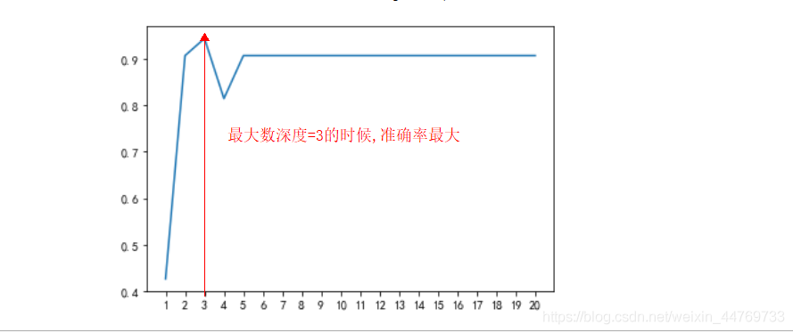
7.4 how to determine the optimal pruning parameters
Here, the learning curve is used to find the optimal parameter with the maximum accuracy / score
Disadvantages: if you need to find the optimal solution of all parameters, you need to nest multi-layer loops, which is very troublesome
Solution: Web search, subsequent updates
Case: use the learning curve to find the optimal solution of the maximum depth
#The data is to be ignored and the case of red wine classification above is to be continued

y=[]
for i in range(1,21):
#4. Establish model
    clf = tree.DecisionTreeClassifier(criterion='gini',
                                random_state=420, #Random seed
                                splitter='random',#Over fitting can be prevented
                                max_depth=i #1. Maximum depth

                                 )
#5. Training model
    clf = clf.fit(Xtrain,Ytrain)
#6. Check accuracy
    score = clf.score(Xtest,Ytest)
    y.append(score)
    print(score) # 0.9444444444444444

#Drawing, learning curve
import matplotlib.pyplot as plt
plt.plot(range(1,21),y)
plt.xticks(range(1,21))
7.5 summary
Attributes are various properties of the model that can be called to view after model training. For the decision tree, the most important is the feature_importances_, Be able to view the importance of each feature to the model.
- The interfaces of many algorithms in sklearn are similar. For example, fit and score, which we have used before, can be used for almost every algorithm. In addition to these two interfaces, the most commonly used interfaces for decision trees are apply and predict.
- Input the test set in apply and return the index of the leaf node where each test sample is located.
- predict the input test set and return the label of each test sample. The returned content is clear at a glance and very easy. If you are interested, you can choose from it
Go down and try. - It must be mentioned here that the input characteristic matrix of all interfaces that require the input of Xtrain and Xtest must be at least one two
Dimensional matrix. sklearn does not accept any one-dimensional matrix as input of characteristic matrix. If your data does have only one feature, it must
Use reshape(-1,1) to add dimension to the matrix. - The classification tree has eight parameters, one attribute, four interfaces, and the code used for drawing:
- Eight parameters: Criterion;
- Two randomness related parameters (random_state, splitter);
- Five pruning parameters (max_depth, min_samples_split, min_samples_leaf, max_feature, min_imparity_decrease);
- One attribute: feature_importances_ ;
- Four interfaces: fit, score, apply, predict
8: Classification model evaluation index (class_weight)
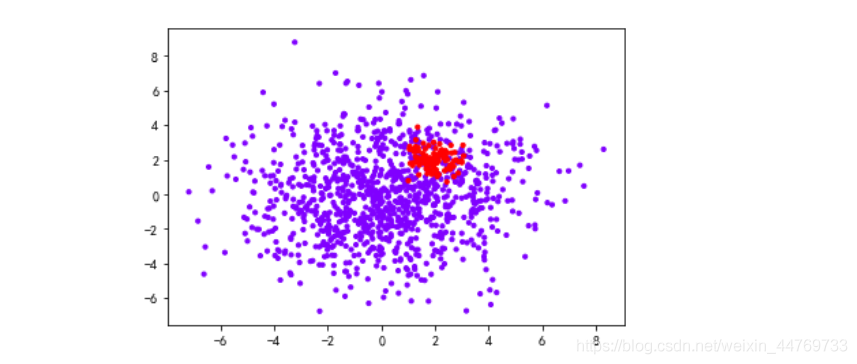
8.1 method of the first sample nonuniformity problem
Create uneven samples
#Case of uneven sample
import numpy as np
import matplotlib.pyplot as plt
from sklearn.tree import DecisionTreeClassifier
from sklearn.datasets import make_blobs #This is the method of clustering to generate data sets

class_1=1000 #Category 1 sample size
class_2=100  #Category 2 sample size
centers=[[0,0],[2,2]] #Center point of two categories
clusters_std=[2.5,0.5] #Variance of two categories

x,y = make_blobs(n_samples=[class_1,class_2],
          centers=centers,
           cluster_std=clusters_std,
           random_state=420,
           shuffle=False
          )

plt.scatter(x[:,0],x[:,1],c=y,cmap='rainbow',s=10)
Comparison setting class_ Score of weight parameter and unset parameter:
#Partition dataset
from sklearn.model_selection import train_test_split
Xtrain,Xtest,Ytrain,Ytest = train_test_split(x,y,test_size=0.2, random_state=420)

#Create model
#1. Do not set class_weight
clf_01 = DecisionTreeClassifier()
clf_01 = clf_01.fit(Xtrain,Ytrain)

score_01 = clf_01.score(Xtest,Ytest)
print('Score without setting parameters=',score_01)
#2. Set class_weight
clf_02 = DecisionTreeClassifier(class_weight='balanced')
clf_02 = clf_02.fit(Xtrain,Ytrain)

score_02 = clf_02.score(Xtest,Ytest)
print('Set the score of the parameter=',score_02)
Result: set class for uneven samples_ Weight can get higher scores
Score without setting parameters= 0.8954545454545455
 Set the score of the parameter= 0.9045454545454545
9: Evaluation index of classification model (confusion matrix – imbalance of special two classification samples)
9.1 concept of confusion matrix
Confusion matrix is a multi-dimensional measurement index system for binary classification problems, which is very useful when the samples are unbalanced
In the confusion matrix, we consider a few classes as positive cases and most classes as negative cases
In the classification algorithms of decision tree and random forest, that is, the minority class is 1 and the majority class is 0
In SVM, that is to say, a few classes are 1 and most classes are - 1
| Estimate | Estimate | ||
|---|---|---|---|
| 1 | 0 | ||
| True value | 1 | 11 (TP) | 10 (FN) |
| True value | 0 | 01 (FP) | 00 (TN) |
Of which:
The row represents the forecast situation, and the column represents the actual situation.
- The predicted value is 1, which is recorded as P (Positive)
- The predicted value is 0 and recorded as N (Negative)
- The predicted value is the same as the real value, which is recorded as T (True)
- The predicted value is opposite to the real value and is recorded as F (False)
- Therefore, the four elements in the matrix represent:
◼ TP (True Positive): the true value is 1, and the predicted value is 1
◼ FN (False Negative): the true value is 1, and the predicted value is 0
◼ FP (False Positive): the true value is 0, and the predicted value is 1
◼ TN (True Negative): the true value is 0, and the predicted value is 0
9.2 model effect evaluation
9.2. 1 Accuracy
Accuracy = (11+00) / (11+00+10+01)
Accuracy is all samples with correct prediction divided by the total samples. Generally speaking, the closer it is to 1, the better.
Remember that a few classes are 1 and most classes are 0
9.2. 2 Precision, also known as Precision
Precision = (11) / (11+01)
Indicates the proportion of the actual number of samples with 1 in all the samples with 1 prediction result.
The lower the accuracy, the greater the proportion of 01, which means that your model has a higher misjudgment rate for most classes 0, and has wrongly injured too many classes (why misjudged most classes? Because most classes are recorded as 0 and a few classes are recorded as 1)
9.2. 3 Recall, also known as sensitivity, real rate and Recall rate
Recall = (11) / (11+10)
Represents the proportion of samples that are predicted to be correct among all samples with a true value of 1
The higher the recall rate, the more minority categories we try to capture
The lower the recall rate, it means that we have not captured enough minority classes
9.2.4 F1 measure
In order to take into account both accuracy and recall, we created the harmonic average of the two as a comprehensive index to consider the balance between the two, which is called F1measure
F-measure = (2 * Precision) / (Precision + Recall)
F1 measure is distributed between [0,1]. The closer it is to 1, the better
9.2. 5 False Negative Rate
It is equal to 1 - Recall. It is used to measure all samples with a real value of 1, which are wrongly judged as 0 by us. It is usually not used much.
FNR = (10) / (11 + 10)
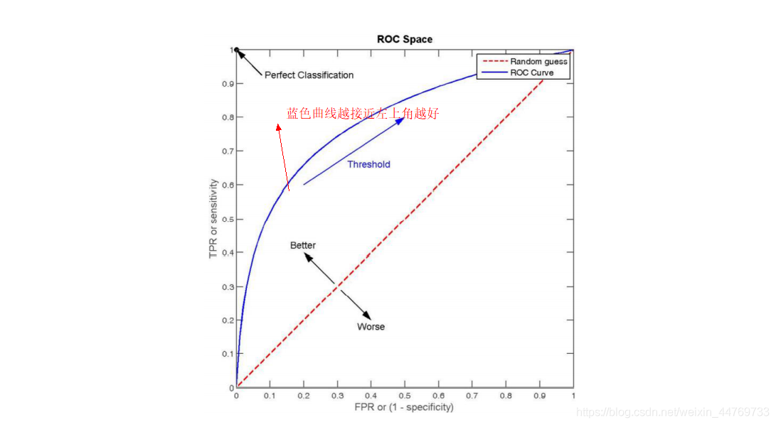
9.2.6 ROC curvereceiver operating characteristic curve
9.3 confusion matrix in sklean
| class | meaning |
|---|---|
| sklearn.metrics.confusion_matrix | Confusion matrix |
| sklearn.metrics.accuracy_score | Accuracy |
| sklearn.metrics.precision_score | accuracy |
| sklearn.metrics.recall_score | recall |
| sklearn.metrics.precision_recall_curve | Accuracy recall balance curve |
| sklearn.metrics.f1_score | F1 measure |
Comparing the two models in the above case, the two models are unbalanced clf_01 / balance CLF_ Some data between 02:
#Import confusion matrix package
from sklearn import metrics

#1. Compare clf_01 and clf_02 accuracy

metrics.precision_score(Ytest,clf_01.predict(Xtest)) #0.6363636363636364

metrics.precision_score(Ytest,clf_02.predict(Xtest)) #0.6538461538461539

#2. Compare recall rate
metrics.recall_score(Ytest,clf_01.predict(Xtest)) #0.4827586206896552
metrics.recall_score(Ytest,clf_02.predict(Xtest)) #0.5862068965517241

#3. Compare F1 value
metrics.f1_score(Ytest,clf_01.predict(Xtest)) #0.5490196078431373
metrics.f1_score(Ytest,clf_02.predict(Xtest)) #0.6181818181818182
10: Advantages and disadvantages of decision tree algorithm
advantage:
- Easy to understand and explain, because trees can be painted and seen.
- Little data preparation is required. Many other algorithms usually need data normalization, creating virtual variables and deleting null values. But please
Note that the decision tree module in sklearn does not support the processing of missing values. - The cost of using the tree (for example, when predicting data) is the logarithm of the number of data points used to train the tree, compared with other algorithms
Law, this is a very low cost. - It can process digital and classified data at the same time, and can do both regression and classification. Other techniques are usually dedicated to analysis with only one
Data set of variable type. - Even if its assumptions violate the real model of generated data to some extent, it can perform well.
Disadvantages:
- Using decision trees may create overly complex trees that do not generalize data well. This is called overfitting. Trimming, setting leaf nodes
Mechanisms such as the minimum number of samples required by points or setting the maximum depth of the tree are necessary to avoid this problem, and the integration and adjustment of these parameters are very important to the beginning
It will be more obscure for scholars. - The decision tree may be unstable, and small changes in the data may lead to completely different trees. This problem needs to be solved by integration algorithm
No. - The learning of decision tree is based on greedy algorithm, which tries to achieve the overall optimization by optimizing the local optimization (the optimization of each node), but this
This method can not guarantee to return to the global optimal decision tree. This problem can also be solved by integrated algorithms in random forests, features and samples
Will be randomly sampled during branching. - If some classes in the tag are dominant, the decision tree learner will create a tree biased towards the dominant class. Therefore, it is suggested to fit the decision tree
Pre balance dataset.