When support vector machine makes decision, the selected decision boundary needs to meet a condition, that is, the distance from the nearest point in the two classifications is the longest. It can also be understood that when we use support vector machine for classification, what we need to do is to maximize the distance between the decision boundary that can distinguish different types of data and the nearest point

This may be difficult to understand. First, let's introduce how to solve the distance from point to plane in support vector machine. Here you can read the solid geometry of high school to deepen your understanding, but the difference is that the dimension is not limited to the two-dimensional plane of high school. Interested readers can read the mathematics textbook of high school to deepen their understanding, Let's use some pictures to strengthen our understanding

，

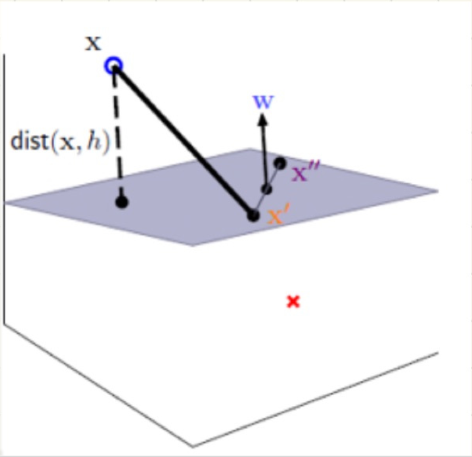
This plane can be understood as the decision boundary you require. To solve the distance from point x to the plane in the graph, we need to use the normal vector of the plane, that is, the W vector in the graph

It can be seen that the equation of the plane is as follows:

Distance from point x to plane

Here, we first describe how to solve the distance from point to plane in support vector machine.

When using support vector machine to solve a simple classification problem, we can understand it with the help of the image above. There are two different data categories above and below the plane. It is certain that there must be a point in each of the two data categories, which is the closest point to the plane in the two data categories.

This paper briefly introduces how to use support vector machine to solve the simple linear classification problem, that is, use a straight line to separate two different data types, so that the shortest distance between this straight line and the two classification data points is the longest. According to the above, the decision boundary is changed into a straight line instead of a plane.

First of all, we need to explain that in the decision boundary equation, W and X are vectors, and the number of elements in the vector depends on the number of features you define. We can also understand several dimensions, because this paper only uses linear classification, only two feature components, two-dimensional space, so w and X have only two elements in this equation.

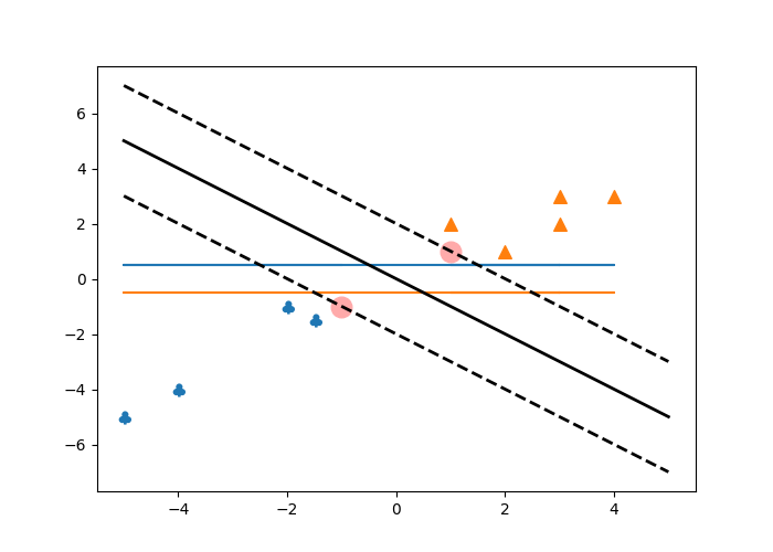
The following program realizes a simple binary classification problem, marks the point closest to the decision boundary with different colors, and uses two dotted lines to reflect the vector machine to maximize the distance between the nearest point and the boundary. The following is the implementation procedure:

import matplotlib.pyplot as plt
import numpy as np
from sklearn.svm import SVC

def plot_svc_decision_boundary(clf, xmin, xmax, sv=True):
    w = clf.coef_
    print(w)
    b = clf.intercept_
    print(b)
    x0 = np.linspace(xmin, xmax, 200)
    decision_boundary = -w[0][0]/w[0][1]*x0 - b/w[0][1]
    margin = 1/w[0][1]
    gutter_up = decision_boundary + margin
    gutter_down = decision_boundary - margin
    if sv:
        svs = clf.support_vectors_
        plt.scatter(svs[:, 0], svs[:, 1], s=180, facecolors='#FFAAAA')
    plt.plot(x0, decision_boundary, 'k-', linewidth=2)
    plt.plot(x0, gutter_up, 'k--', linewidth=2)
    plt.plot(x0, gutter_down, 'k--', linewidth=2)
    plt.show()
X = np.array([[-1.0, -1.0], [-1.5, -1.5], [-5, -5],[-4, -4], [-2.0, -1.0], [1.0, 1.0], [2.0, 1.0], [3.0, 2.0], [1.0, 2.0], [4.0, 3.0], [3.0, 3.0]])
y = [1, 1, 1, 1, 1, 2, 2, 2, 2, 2, 2]#    Tag value corresponding to X data
x0 = [X[0][0], X[1][0], X[2][0], X[3][0], X[4][0], X[5][0], X[6][0], X[7][0], X[8][0], X[9][0], X[10][0]]
y0 = [X[0][1], X[1][1], X[2][1], X[3][1], X[4][1], X[5][1], X[6][1], X[7][1], X[8][1], X[9][1], X[10][1]]
x1 = [X[0][0], X[1][0], X[2][0], X[3][0], X[4][0]]
y1 = [X[0][1], X[1][1], X[2][1], X[3][1], X[4][1]]
plt.figure(figsize=(7, 5))
plt.scatter(x1, y1, s=70, marker='$\clubsuit$')
x2 = [X[5][0], X[6][0], X[7][0], X[8][0], X[9][0], X[10][0]]
y2 = [X[5][1], X[6][1], X[7][1], X[8][1], X[9][1], X[10][1]]
y3 = [0.5, 0.5, 0.5, 0.5, 0.5, 0.5, 0.5, 0.5, 0.5, 0.5, 0.5]
y4 = [-0.5, -0.5, -0.5, -0.5, -0.5, -0.5, -0.5, -0.5, -0.5, -0.5, -0.5]
plt.scatter(x2, y2, s=70, marker='^')
plt.plot(x0, y3)
plt.plot(x0, y4)
clf = SVC(kernel='linear', C=float('inf'))
clf.fit(X, y)
plot_svc_decision_boundary(clf, -5, 5)
plt.show()
print(clf.predict([[3, 2]]))

This is the effect diagram of the implementation:

At the same time, there are two lines with different colors, which can be understood as the decision line realized by the traditional classification method.

The last command print(clf.predict([[3, 2]])) realizes the result value of the prediction of the given data, and the result value belongs to the defined label range.