Ex6_ Machine learning_ Wu Enda course assignment (Python): SVM Support Vector Machines
instructions:
This article is about Mr. Wu Enda's learning notes of the machine learning course on Coursera.
- The first part of this paper first introduces the knowledge review and key notes of the corresponding week of the course, as well as the introduction of the code implementation library.
- The second part of this paper includes the implementation details of user-defined functions in the code implementation part.
- The third part of this paper is the specific code implementation corresponding to the course practice topic.
0. Pre-condition
This section includes some introductions of libraries.
# This file includes self-created functions used in exercise 3
import numpy as np
import matplotlib.pyplot as plt
import scipy.optimize as opt
from scipy.io import loadmat
00. Self-created Functions
This section includes self-created functions.
-
loadData(path): read data
# Load data from the given file # Args: {path: data path} def loadData(path): data = loadmat(path) return data['X'], data['y'] -
plotData(X, y): visual data
# Visualize data # Args: {X: training set; y: tag set} def plotData(X, y): plt.figure(figsize=[8, 6]) plt.scatter(X[:, 0], X[:, 1], c=y.flatten()) plt.xlabel('X1') plt.ylabel('X2') plt.title('Data Visualization') # plt.show() -
Plot boundary (classifier, x): draw the decision boundary between categories
# Plot the boundary between two classes # Args: {classifier: classifier; X: training set} def plotBoundary(classifier, X): x_min, x_max = X[:, 0].min() * 1.2, X[:, 0].max() * 1.1 y_min, y_max = X[:, 1].min() * 1.2, X[:, 1].max() * 1.1 xx, yy = np.meshgrid(np.linspace(x_min, x_max, 500), np.linspace(y_min, y_max, 500)) # Use the incoming classifier to make category prediction for the prediction samples Z = classifier.predict(np.c_[xx.flatten(), yy.flatten()]) Z = Z.reshape(xx.shape) plt.contour(xx, yy, Z) -
displayBoundaries(X, y): draw the decision boundary (linear kernel) under different SVM parameters C
# Display boundaries for different situations with different C (1 and 100) # Change the SVM parameter C and draw the decision boundary in each case # Args: {X: training set; y: tag set} def displayBoundaries(X, y): # Here, skilearn's package is used to obtain multiple SVM models by using linear kernel function models = [svm.SVC(C=C, kernel='linear') for C in [1, 100]] # Given the training set X and label set y, multiple SVM models are trained to obtain multiple classifiers classifiers = [model.fit(X, y.flatten()) for model in models] # Output information titles = ['SVM Decision Boundary with C = {}'.format(C) for C in [1, 100]] # For each classifier, draw its decision boundary for classifier, title in zip(classifiers, titles): plotData(X, y) plotBoundary(classifier, X) plt.title(title) # Display data plt.show() -
Gaussian kernel (x1, X2, sigma): realize Gaussian kernel function

# Implement a Gaussian kernel function (Could be considered as a similarity function) # Realize Gaussian kernel function (which can be regarded as similarity function to measure the distance between a pair of samples) # Args: {X1: sample 1; x2: Sample 2; sigma: Gaussian kernel function parameter} def gaussianKernel(x1, x2, sigma): return np.exp(-(np.power(x1 - x2, 2).sum() / (2 * np.power(sigma, 2)))) -
displayGaussKernelBoundary(X, y, C, sigma): draw the decision boundary of Gaussian kernel SVM for a data set
# Display the decision boundary using SVM with a Gaussian kernel # Draw the decision boundary of SVM based on Gaussian kernel for a data set # Args: {X: training set; y: label set; C: SVM parameter; sigma: Gaussian kernel function parameter} def displayGaussKernelBoundary(X, y, C, sigma): gamma = np.power(sigma, -2.) / 2 # 'rbf' refers to radial basis function / Gaussian kernel function model = svm.SVC(C=1, kernel='rbf', gamma=gamma) classifier = model.fit(X, y.flatten()) plotData(X, y) plotBoundary(classifier, X) plt.title('Decision boundary using SVM with a Gaussian Kernel') plt.show() -
trainGaussParams(X, y, Xval, yval): compare the error of cross validation set and train the optimal parameters C and sigma
# Train out the best parameters 'C' and 'sigma" with the least cost on the validation set # By comparing the errors in the cross validation set, the optimal parameters C and sigma are trained # Args: {X: training set; y: tag set; Xval: training cross validation set; yval: tag cross validation set} def trainGaussParams(X, y, Xval, yval): C_values = (0.01, 0.03, 0.1, 0.3, 1., 3., 10., 30.) sigma_values = C_values best_pair, best_score = (0, 0), 0 for C in C_values: for sigma in sigma_values: gamma = np.power(sigma, -2.) / 2 model = svm.SVC(C=C, kernel='rbf', gamma=gamma) classifier = model.fit(X, y.flatten()) this_score = model.score(Xval, yval) if this_score > best_score: best_score = this_score best_pair = (C, sigma) print('Best pair(C, sigma): {}, best score: {}'.format(best_pair, best_score)) return best_pair[0], best_pair[1] -
Preprocess email (email): preprocess mail
# Preprocess an email # Performs all processing except Word Stemming and removal of non words def preprocessEmail(email): # Full text lowercase email = email.lower() # Unify HTML format. Matching the beginning of < and all contents that are not <, > until the end of > is equivalent to matching <... > email = re.sub('<[^<>]>', ' ', email) # Unify URLs. Convert all URL addresses to "httpadddr". email = re.sub('(http|https)://[^\s]*', 'httpaddr', email) # Unified email address. Convert all email addresses to "emailaddr". email = re.sub('[^\s]+@[^\s]+', 'emailaddr', email) # Unify dollar sign. email = re.sub('[\$]+', 'dollar', email) # Unify numbers. email = re.sub('[\d]+', 'number', email) return email -
email2TokenList(email): extract the stem and remove the non character content to return the word list
# Conduct Word Stemming and Removal of non-words. # Besides, here we use "NLTK" lib's stemmer, since it's more accurate and efficient. # Perform the processing of stem extraction and removing non character content, and return the processed words one by one # The extractor of NLTK package is used here, which is more efficient and accurate def email2TokenList(email): # Preprocess the email email = preprocessEmail(email) # Instantiate the stemmer stemmer = nltk.stem.porter.PorterStemmer() # Split the whole email into separated words tokens = re.split('[ \@\$\/\#\.\-\:\&\*\+\=\[\]\?\!\(\)\{\}\,\'\"\>\_\<\;\%]', email) # Traverse all the split contents token_list = [] for token in tokens: # Remove non word contents deletes any non alphanumeric characters token = re.sub('[^a-zA-Z0-9]', '', token) # Stem the root of the word stemmed_word = stemmer.stem(token) # Remove empty string removes the empty string '', which does not contain any characters. It is not added if not len(token): continue # Append the word into the list token_list.append(stemmed_word) return token_list -
email2VocabularyList(email, vocab_list): get the index of words appearing in both email and vocabulary
# Get the indices of words that exist both in the email and the vocabulary list # Gets the index of words that appear simultaneously in the message and vocabulary # Args: {email: mail; vocab_list: word list} def email2VocabularyList(email, vocab_list): token = email2TokenList(email) index = [i for i in range(len(vocab_list)) if vocab_list[i] in token] return index -
email2FeatureVector(email): extract features of email
# Extract features from email, turn the email into a feature vector
# Extract the features of the mail and obtain a feature vector representing the mail (the length is the length of the word list. If the word exists, the corresponding subscript position value is 1, otherwise it is 0)
# Args: {email:}
def email2FeatureVector(email):
    # Word list provided
    df = pd.read_table('../data/vocab.txt', names=['words'])
    vocab_list = np.asmatrix(df)
    # The length is the same as that of the word list
    feature_vector = np.zeros(len(vocab_list))
    # If the word exists in the email, the corresponding subscript position value is 1, otherwise it is 0
    vocab_indices = email2VocabularyList(email, vocab_list)
    for i in vocab_indices:
        feature_vector[i] = 1
    return feature_vector
1. Support Vector Machines
In the fifirst half of this exercise, you will be using support vector machines (SVMs) with various example 2D datasets.
Experimenting with these datasets will help you gain an intuition of how SVMs work and how to use a Gaussian kernel with SVMs.
In the next half of the exercise, you will be using support vector machines to build a spam classififier.
- The relevant functions called are described in detail in the article header "self created functions".
# 1. Support Vector Machines
path = '../data/ex6data1.mat'
X, y = func.loadData(path)
1.1 Example dataset 1
# 1.1 Example dataset 1
# Visual data
func.plotData(X, y)

# Try different parameters C and draw the decision boundary in various cases
func.displayBoundaries(X, y)
-
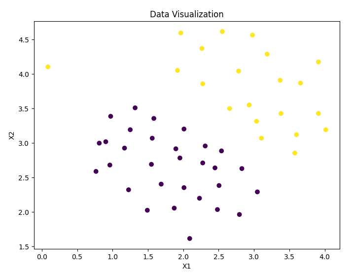
Data visualization:
-
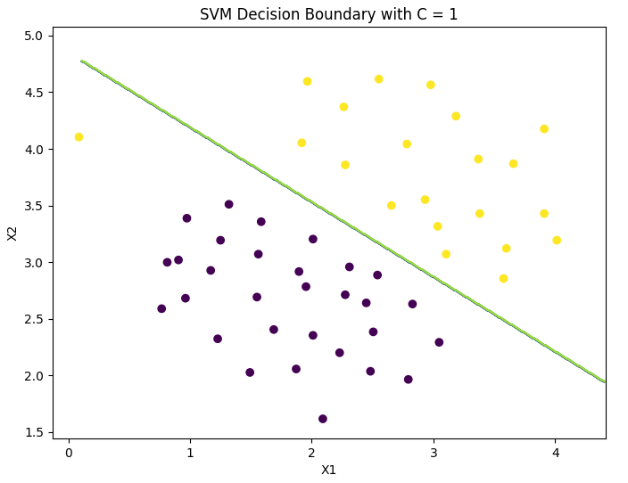
Decision boundary (linear kernel, C = 1):
-
Decision boundary (linear kernel, C = 100):
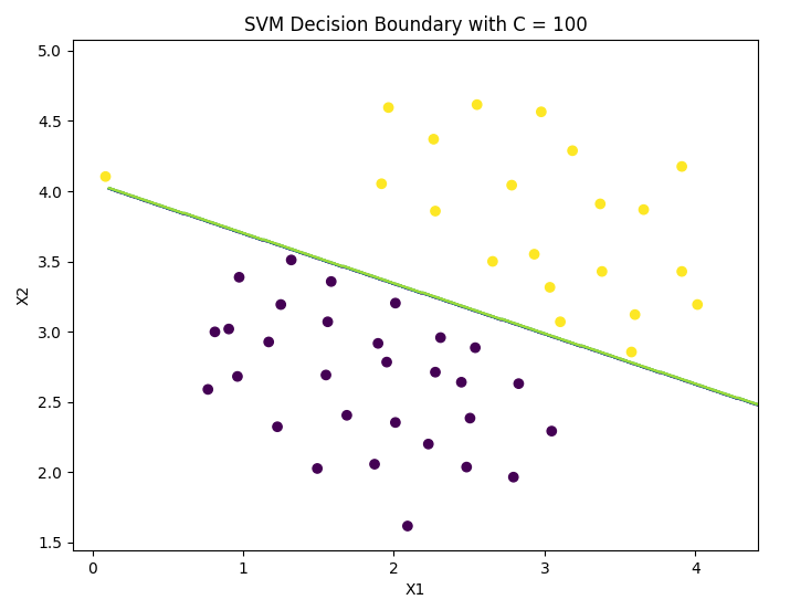
As can be seen from the above figure:
- When C C C) larger (i.e 1 / λ 1/\lambda 1/ λ Larger, λ \lambda λ When it is small, the punishment of misclassification by the model increases, which is more strict, less misclassification and smaller interval.
- When C C C) smaller (i.e 1 / λ 1/\lambda 1/ λ Smaller, λ \lambda λ When it is large, the punishment of misclassification by the model is reduced and loose, allowing a certain misclassification to exist with a large interval.
1.2 SVM with Gaussian Kernels
In order to find the nonlinear decision boundary with SVM, we first need to implement Gaussian kernel function. I can think of Gaussian kernel function as a similarity function to measure the distance between a pair of samples ( x ( i ) , y ( j ) ) (x^{(i)}, y^{(j)}) (x(i),y(j)).
Note that most SVM libraries will automatically add additional features for you x 0 x_0 x0 , and θ 0 \theta_0 θ 0, so there is no need to add it manually.
# 1.2 SVM with Gaussian Kernels SVM based on Gaussian kernel function
path2 = '../data/ex6data2.mat'
X2, y2 = func.loadData(path2)

path3 = '../data/ex6data3.mat'
df3 = loadmat(path3)
X3, y3, Xval, yval = df3['X'], df3['y'], df3['Xval'], df3['yval']
1.2.1 Gaussian Kernel

# 1.2.1 Gaussian Kernel Gaussian kernel function
res_gaussianKernel = func.gaussianKernel(np.array([1, 2, 1]), np.array([0, 4, -1]), 2.)
print(res_gaussianKernel)  # 0.32465246735834974
1.2.2 Example dataset 2
# 1.2.2 Example dataset 2
# Visual data
func.plotData(X2, y2)

# Draw the decision boundary of SVM based on Gaussian kernel function for data set
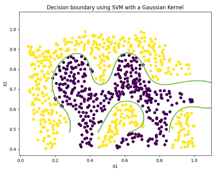
func.displayGaussKernelBoundary(X2, y2, C=1, sigma=0.1)
-
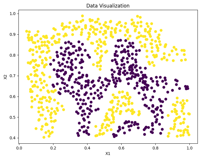
Data visualization:
-
Decision boundary (Gaussian kernel):
1.2.3 Example dataset 3
# 1.2.3 Example dataset 3
# Visual data
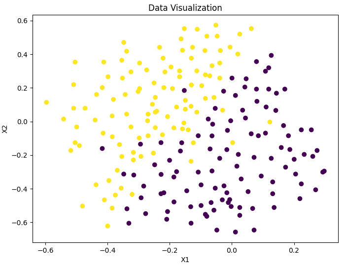
func.plotData(X3, y3)

# Training parameters C and sigma of SVM based on Gaussian kernel function
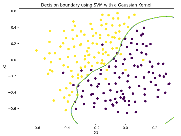
final_C, final_sigma = func.trainGaussParams(X3, y3, Xval, yval)

# Draw the decision boundary of SVM based on Gaussian kernel function for data set
func.displayGaussKernelBoundary(X3, y3, C=final_C, sigma=final_sigma)
-
Data visualization:
-
Decision boundary (Gaussian kernel, optimal parameter):
2. Spam Classification
This section includes some details of exploring "Spam Classification" using SVM.
- The relevant functions called are described in detail in the article header "self created functions".
In this part, we will use SVM to establish a spam classifier. You need to turn every email into one n n The classifier will judge the given e-mail based on the n # dimensional feature vector x x x # is spam ( y = 1 ) (y = 1) (y=1) or not spam ( y = 0 ) (y = 0) (y=0).
# 2. Spam Classifier
# Get mail content
with open('../data/emailSample1.txt', 'r') as f:
    email = f.read()
    print(email)
2.1 Preprocess Emails
You can see that the email content includes URL, email address, number and dollar symbol. Many emails contain these elements, but the specific content of each email may be different. Therefore, when dealing with mail, the method often used is to standardize data, that is, treat all URLs as the same, all numbers as the same, etc.
For example, we replace all URLs with a unique string 'httpaddr' to indicate that the email contains a URL without requiring specific URL content. This usually improves the performance of the spam classifier because spammers usually randomize URLs, so the chance of seeing any specific URL again in new spam is very small.
We can do the following:
- Lower casting: convert the whole message to lowercase.
- Stripping HTML: remove all HTML tags and keep only the content.
- Normalizing URLs: replace all URLs with the string "httpaddr"
- Normalizing Email Addresses: replace all addresses with "emailaddr"
- Normalizing Dollars: replace all dollar symbols ($) with "dollar"
- Normalizing Numbers: replace all numbers with "number"
- Word stemming: restore all words to etymology. For example, "discount", "discounts", "discounted" and "discounting" are replaced by "discount".
- Removal of non words: remove all non text types and adjust all spaces (tabs, newlines, spaces) to one space
See the user-defined function section at the head of the article for the specific code.
# 2.1 Preprocess emails
# 2.1.1 Vocabulary List
# 2.2 Extract Features from emails
feature_vector = func.email2FeatureVector(email)
print('Length of feature vector = {}\nNumber of occurred words = {}'
      .format(len(feature_vector), int(feature_vector.sum())))
Output result:
Length of feature vector = 1899
Number of occurred words = 45
2.1.1 Vocabulary List
After preprocessing the mail, we get the processed word list. Next, we choose the words we use in the classifier and which words we need to remove.
The title provides a glossary vocab Txt, which contains 1899 words often used in practice.
We need to figure out how much vocab is in the processed email Txt and returns the word in vocab Txt, that is, the index of the training words we want.
2.2 Extract Features from Emails
Extract the features of the mail and obtain a feature vector representing the mail (the length is the length of the word list, and the corresponding subscript position value is if the word exists) 1 1 1. Otherwise 0 0 0 ).
2.3 Train SVM for Spam Classification
Read the extracted feature vector and the corresponding label. It is divided into training set and test set.
# 2.3 Train SVM for Spam Classification
# Read the extracted feature vector and the corresponding label. It is divided into training set and test set.
path_train = '../data/spamTrain.mat'
path_test = '../data/spamTest.mat'
mat_train = loadmat(path_train)
mat_test = loadmat(path_test)
X_train, y_train = mat_train['X'], mat_train['y']
X_test, y_test = mat_test['Xtest'], mat_test['ytest']
# Fit the model training model
model = svm.SVC(C=0.1, kernel='linear')
model.fit(X_train, y_train)
2.4 Top Predictiors for Spam
# 2.4 significant indicators of top predictors for spam
prediction_train = model.score(X_train, y_train)
prediction_test = model.score(X_test, y_test)
print('Predictions of training: ', prediction_train)
print('Predictions of testing: ', prediction_test)
Output result:
Predictions of training: 0.99825
Predictions of testing: 0.989