At present, the updated part includes the basic setting, basic module, relative position coordinate understanding and some code display of swin.
swin contains four setting s, tiny, small, base and large. It can be compared to resnet.
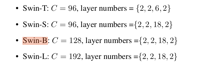
Swin-b main part network structure BasicLayer
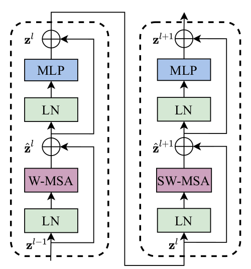
Structure display
BasicLayer(
  (blocks): ModuleList(

    (0): SwinTransformerBlock(
      (norm1): LayerNorm((128,), eps=1e-05, elementwise_affine=True)
      # WindowAttention
      (attn): WindowAttention(
        (qkv): Linear(in_features=128, out_features=384, bias=True)
        (attn_drop): Dropout(p=0.0, inplace=False)
        (proj): Linear(in_features=128, out_features=128, bias=True)
        (proj_drop): Dropout(p=0.0, inplace=False)
        (softmax): Softmax(dim=-1)
      )
      (drop_path): Identity()
      (norm2): LayerNorm((128,), eps=1e-05, elementwise_affine=True)
      (mlp): Mlp(
        (fc1): Linear(in_features=128, out_features=512, bias=True)
        (act): GELU()
        (fc2): Linear(in_features=512, out_features=128, bias=True)
        (drop): Dropout(p=0.0, inplace=False)
      )
    )


    (1): SwinTransformerBlock(
      (norm1): LayerNorm((128,), eps=1e-05, elementwise_affine=True)
      (attn): WindowAttention(
        (qkv): Linear(in_features=128, out_features=384, bias=True)
        (attn_drop): Dropout(p=0.0, inplace=False)
        (proj): Linear(in_features=128, out_features=128, bias=True)
        (proj_drop): Dropout(p=0.0, inplace=False)
        (softmax): Softmax(dim=-1)
      )
      (drop_path): DropPath()
      (norm2): LayerNorm((128,), eps=1e-05, elementwise_affine=True)
      (mlp): Mlp(
        (fc1): Linear(in_features=128, out_features=512, bias=True)
        (act): GELU()
        (fc2): Linear(in_features=512, out_features=128, bias=True)
        (drop): Dropout(p=0.0, inplace=False)
      )
    )
  )


  (downsample): PatchMerging(
    (reduction): Linear(in_features=512, out_features=256, bias=False)
    (norm): LayerNorm((512,), eps=1e-05, elementwise_affine=True)
  )
)
Whole flow chart
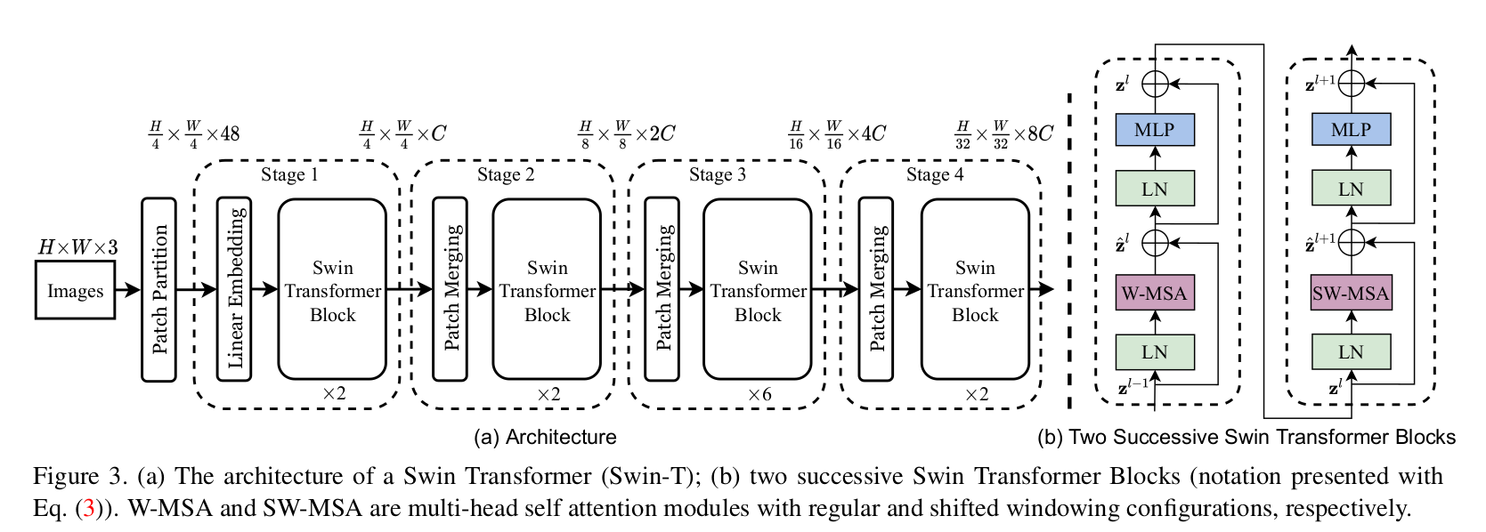
Non overlap patch partition module in Vit mode
First, pad to an integer multiple of the patch size
if W % self.patch_size[1] != 0:
    x = F.pad(x, (0, self.patch_size[1] - W % self.patch_size[1]))
if H % self.patch_size[0] != 0:
    x = F.pad(x, (0, 0, 0, self.patch_size[0] - H % self.patch_size[0]))
The core is to use a conv with stripe instead of sub patch operation.
#using a nxn (s=n) conv is equivalent to splitting nxn (no overlap) patches.
self.proj = nn.Conv2d(in_chans, embed_dim, kernel_size=patch_size, stride=patch_size)
if norm_layer is not None:
    self.norm = norm_layer(embed_dim)
else:
    self.norm = None
The feature obtained by encoding is the feature obtained by patch encoding.
Partition windows modules
After the embedding obtained by patch coding is obtained, it is divided by window in the following way. Different windows are placed on the batch axis for convenient and fast calculation.
# partition windows, nW means number of windows
x_windows = window_partition(
    shifted_x, self.window_size
)  # nW*B, window_size, window_size, C    [392, 12, 12, 128]
x_windows = x_windows.view(
    -1, self.window_size * self.window_size, C
)  # nW*B, window_size*window_size, C
WindowAttention module
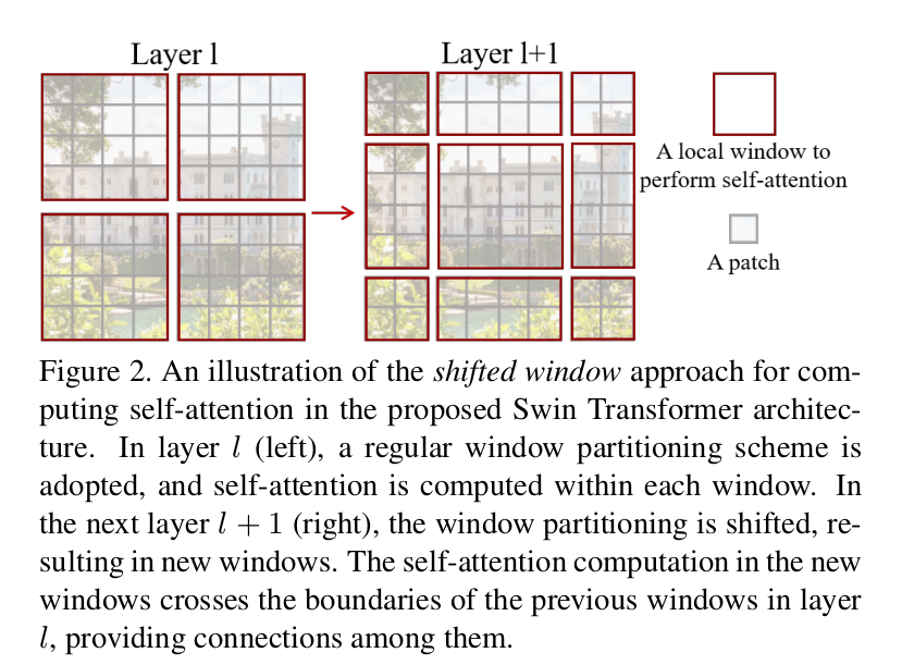
Here is the essence of swin. The author also compares the complexity of global computing affinity and sliding window computing
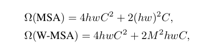
Here M is the window size constant. Next, let's explain the code module.
Suppose some super parameters
self.window_size = window_size  # Wh, Ww, (12, 12)
self.num_heads = num_heads # 4
head_dim = dim // num_heads # 32
self.scale = qk_scale or head_dim ** -0.5 # 0.17
Learnable relative position coding
Create a learnable embedding with a size of [(2* Wh-1) * (2* Ww-1), nH]. Why is the size like this? This is because you need to look up table, that is, look up table to get the weight of a position. Here's an explanation, because a table needs to include a solution space. The solution space (2* Wh-1) * (2* Ww-1) is so large, and then it is used as an index, that is, a subscript to index the relative_position_bias_table. For example, if two embedded spaces are 10 apart, you need to find relative_position_bias_table [10], with a distance of - 10, is relative_position_bias_table [-10].
# define a parameter table of relative position bias
self.relative_position_bias_table = nn.Parameter(
    torch.zeros((2 * window_size[0] - 1) * (2 * window_size[1] - 1), num_heads)
)  # 2*Wh-1 * 2*Ww-1, nH (denotes num_heads)
Relative position table
You need to generate a relative coordinate code of 12 x 12 window. Think about how much solution space can cover the relative position? When the 12x12 window is simply described by the coordinate position difference for each line, it is [- 11, 11], that is, 2w-1 values. The positive and negative are because the relative positions before and after are not undirected. The target matrix size is (2w-1)x(2h-1). Well, if you know what we want to do, it's up to the code.
Get a coords first_ Flat, the size is (2, Wh * Ww), and W represents window.
tensor([[ 0,  0,  0,  0,  0,  0,  0,  0,  0,  0,  0,  0,  1,  1,  1,  1,  1,  1,
          1,  1,  1,  1,  1,  1,  2,  2,  2,  2,  2,  2,  2,  2,  2,  2,  2,  2,
          3,  3,  3,  3,  3,  3,  3,  3,  3,  3,  3,  3,  4,  4,  4,  4,  4,  4,
          4,  4,  4,  4,  4,  4,  5,  5,  5,  5,  5,  5,  5,  5,  5,  5,  5,  5,
          6,  6,  6,  6,  6,  6,  6,  6,  6,  6,  6,  6,  7,  7,  7,  7,  7,  7,
          7,  7,  7,  7,  7,  7,  8,  8,  8,  8,  8,  8,  8,  8,  8,  8,  8,  8,
          9,  9,  9,  9,  9,  9,  9,  9,  9,  9,  9,  9, 10, 10, 10, 10, 10, 10,
         10, 10, 10, 10, 10, 10, 11, 11, 11, 11, 11, 11, 11, 11, 11, 11, 11, 11],
        [ 0,  1,  2,  3,  4,  5,  6,  7,  8,  9, 10, 11,  0,  1,  2,  3,  4,  5,
          6,  7,  8,  9, 10, 11,  0,  1,  2,  3,  4,  5,  6,  7,  8,  9, 10, 11,
          0,  1,  2,  3,  4,  5,  6,  7,  8,  9, 10, 11,  0,  1,  2,  3,  4,  5,
          6,  7,  8,  9, 10, 11,  0,  1,  2,  3,  4,  5,  6,  7,  8,  9, 10, 11,
          0,  1,  2,  3,  4,  5,  6,  7,  8,  9, 10, 11,  0,  1,  2,  3,  4,  5,
          6,  7,  8,  9, 10, 11,  0,  1,  2,  3,  4,  5,  6,  7,  8,  9, 10, 11,
          0,  1,  2,  3,  4,  5,  6,  7,  8,  9, 10, 11,  0,  1,  2,  3,  4,  5,
          6,  7,  8,  9, 10, 11,  0,  1,  2,  3,  4,  5,  6,  7,  8,  9, 10, 11]])
Then use
relative_coords = coords_flatten[:, :, None] - coords_flatten[:, None, :] # 2, Wh*Ww, Wh*Ww
coords_ Flat [:,:, none] dimension is [2, 144, 1], coords_flatten[:, None,:] dimension is [2, 1, 144]
The two matrices are subtracted correspondingly, and the relative position is obtained according to the broadcast rules. relative_coords dimensions [2, 144144]. Broadcast rules can be seen as fixed coords_ The first element of flatten [0] is 0, followed by coords_ Subtract each element of flatten [1].
tensor([[[  0,   0,   0,  ..., -11, -11, -11],
         [  0,   0,   0,  ..., -11, -11, -11],
         [  0,   0,   0,  ..., -11, -11, -11],
         ...,
         [ 11,  11,  11,  ...,   0,   0,   0],
         [ 11,  11,  11,  ...,   0,   0,   0],
         [ 11,  11,  11,  ...,   0,   0,   0]],

        [[  0,  -1,  -2,  ...,  -9, -10, -11],
         [  1,   0,  -1,  ...,  -8,  -9, -10],
         [  2,   1,   0,  ...,  -7,  -8,  -9],
         ...,
         [  9,   8,   7,  ...,   0,  -1,  -2],
         [ 10,   9,   8,  ...,   1,   0,  -1],
         [ 11,  10,   9,  ...,   2,   1,   0]]])
We can roughly calculate that the minimum is 0-11 = - 11 and the maximum is 11-0 = 11, which is in line with our expectations. At this time, the index contains many negative values. At this time, we can offset all negative numbers by + 11 in each direction. At this time, the maximum value is 22 and the minimum value is 0
relative_coords[:, :, 0] += self.window_size[0] - 1  # shift to start from 0
relative_coords[:, :, 1] += self.window_size[1] - 1
In swin, relative position coding acts as B, that is, bias when calculating similarity. In order to change the above two-dimensional relative position matrix into one-dimensional
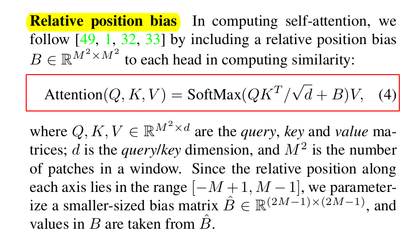 , the simplest way is to encode i* (2w-1)+j. swin adopts an efficient implementation.
relative_coords[:, :, 0] *= 2 * self.window_size[1] - 1
# The lower axis passes through permute(1, 2, 0), putting 2 at the end
relative_position_index = relative_coords.sum(-1)  # Wh*Ww, Wh*Ww
So the final maximum value is 22 x (2x12-1) + 22 = 528, and the minimum value is 0. Notice that w is 12, and i, j adds a paranoid 11, so it becomes the maximum 22.
Summary
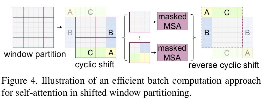
The purpose of sliding window can be achieved by cyclic displacement.