Reference source: https://github.com/datawhalechina/team-learning-data-mining/tree/master/EnsembleLearning

1. Data set

1.1 background introduction

The basic principle of thermal power generation is: when the fuel is burned, it heats water to generate steam, the steam pressure drives the steam turbine to rotate, and then the steam turbine drives the generator to rotate to generate electric energy. In this series of energy conversion, the core affecting the power generation efficiency is the combustion efficiency of the boiler, that is, fuel combustion heats water to produce high-temperature and high-pressure steam. There are many factors affecting the combustion efficiency of the boiler, including the adjustable parameters of the boiler, such as combustion feed, primary and secondary air, induced air, return air and water supply; And the working conditions of the boiler, such as boiler bed temperature and bed pressure, furnace temperature and pressure, superheater temperature, etc. How can we use the above information to predict the amount of steam produced according to the working conditions of the boiler, so as to contribute to the output prediction of China's industrial industry?

Therefore, this case is to use the characteristics of the above industrial indicators to predict the steam volume. Due to information security and other reasons, we use the data collected by the desensitized boiler sensor (the acquisition frequency is minute level).

In fact, it doesn't seem to have anything to do with this background, because it's desensitized data. We don't know what the real meaning of each attribute is, so we don't need to manually process each attribute, add artificial attributes and cross attributes, etc.

1.2 data set

The data is divided into training data (train.txt) and test data (test.txt), in which the fields "V0" - "V37" are used as characteristic variables and "target" is used as target variables. We need to use the training data to train the model and predict the target variables of the test data.

1.3 evaluation index:

The final evaluation index is the mean square error MSE, namely:
S c o r e = 1 n ∑ 1 n ( y i − y ∗ ) 2 Score = \frac{1}{n} \sum_1 ^n (y_i - y ^*)^2 Score=n1​1∑n​(yi​−y∗)2

2. Data preprocessing

2.1 importing dependent packages

import warnings
warnings.filterwarnings("ignore")
import matplotlib.pyplot as plt
import seaborn as sns

# Model
import pandas as pd
import numpy as np
from scipy import stats
from sklearn.model_selection import train_test_split
from sklearn.model_selection import GridSearchCV, RepeatedKFold, cross_val_score,cross_val_predict,KFold
from sklearn.metrics import make_scorer,mean_squared_error
from sklearn.linear_model import LinearRegression, Lasso, Ridge, ElasticNet
from sklearn.svm import LinearSVR, SVR
from sklearn.neighbors import KNeighborsRegressor
from sklearn.ensemble import RandomForestRegressor, GradientBoostingRegressor,AdaBoostRegressor
from xgboost import XGBRegressor
from sklearn.preprocessing import PolynomialFeatures,MinMaxScaler,StandardScaler

2.2 reading data

data_train = pd.read_csv('train.txt',sep = '\t')
data_test = pd.read_csv('test.txt',sep = '\t')

#Merge training data and test data
#Before merging training data and test data, label them to indicate the source
data_train["oringin"]="train"
data_test["oringin"]="test"
data_all=pd.concat([data_train,data_test],axis=0,ignore_index=True)
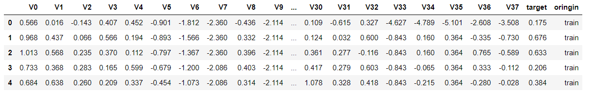
#Display the first 5 data
data_all.head()

2.3 exploratory analysis of data

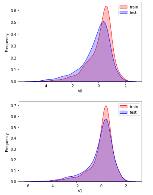
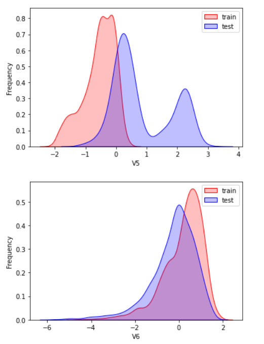
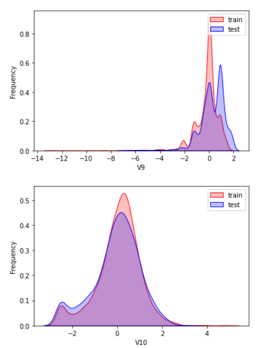
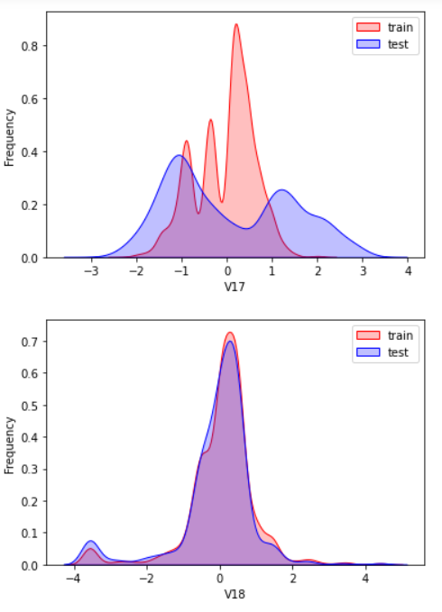
Here, kdeplot (nuclear density estimation map) is used for preliminary analysis of data, namely EDA.

Kernel density estimation
Nuclear density estimation: https://www.zhihu.com/question/27301358

According to my understanding, the kernel density estimation is to know the scatter diagram and make regression. The connection is required to be as smooth as possible and roughly observe the distribution of the data. In this example, the distribution of training set and test set data is observed through kernel density estimation, so as to delete attribute values that do not have similar distribution.

for column in data_all.columns[0:-2]:
    #Kernel density estimation is used to estimate the unknown density function in probability theory. It is one of the nonparametric test methods. Through the kernel density estimation diagram, we can intuitively see the distribution characteristics of the data samples themselves.
    #kdeplot Manual: https://www.cntofu.com/book/172/docs/25.md
    #ax: the coordinate axis to be drawn. If it is empty, the current axis will be used
    g = sns.kdeplot(data_all[column][(data_all["oringin"] == "train")], color="Red", shade = True)
    g = sns.kdeplot(data_all[column][(data_all["oringin"] == "test")], ax =g,color="Blue", shade= True)
    g.set_xlabel(column)
    g.set_ylabel("Frequency")
    g = g.legend(["train","test"])
    plt.show()

There are too many pictures. Select some typical data for observation




View the correlation between features (degree of correlation)

#Draw thermal map
#The thermal map does not contain the origin attribute
data_train1=data_all[data_all["oringin"]=="train"].drop("oringin",axis=1)
plt.figure(figsize=(20, 20))  # Specifies the width and height of the drawing object
colnm = data_train1.columns.tolist()  # List header
mcorr = data_train1[colnm].corr(method="spearman")  # The correlation coefficient matrix gives the correlation coefficient between any two variables
mask = np.zeros_like(mcorr, dtype=np.bool)  # It is constructed that the number matrix with the same dimension as mcorr is bool type
mask[np.triu_indices_from(mask)] = True  # True to the right of the corner divider
cmap = sns.diverging_palette(220, 10, as_cmap=True)  # Return matplotlib colormap object, color palette
g = sns.heatmap(mcorr, mask=mask, cmap=cmap, square=True, annot=True, fmt='0.2f')  # Thermodynamic diagram (see two similarity)
plt.show()

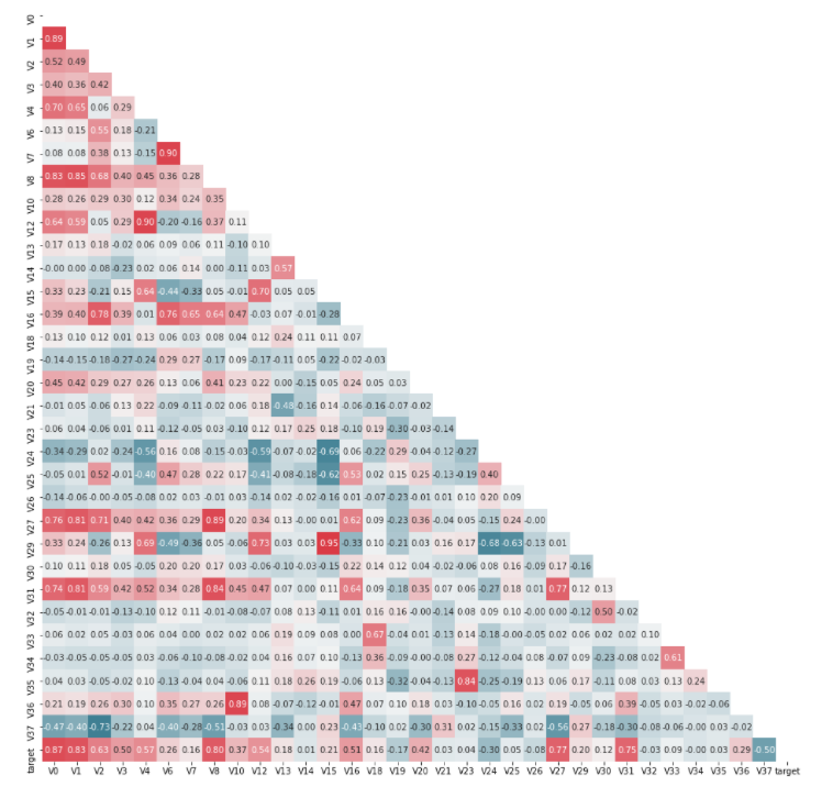
Dimensionality reduction operation, that is, delete the features whose absolute value of correlation is less than the threshold

threshold = 0.1
corr_matrix = data_train1.corr().abs()
drop_col=corr_matrix[corr_matrix["target"]<threshold].index
data_all.drop(drop_col,axis=1,inplace=True)

Then normalize the formula:
y = c o l − c o l . m i n ( ) c o l . m a x ( ) − c o l . m i n ( ) y = \frac {col-col.min()}{col.max()-col.min()} y=col.max()−col.min()col−col.min()​

cols_numeric=list(data_all.columns)
cols_numeric.remove("oringin")

def scale_minmax(col):
    return (col-col.min())/(col.max()-col.min())

scale_cols = [col for col in cols_numeric if col!='target']
data_all[scale_cols] = data_all[scale_cols].apply(scale_minmax,axis=0)
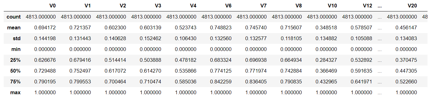
data_all[scale_cols].describe()

#After normalization, the maximum value must be 1. According to the formula
#According to the formula, the minimum value must be 0 after normalization

The above is to complete the whole process of data processing. However, missing values and outliers are not filled in this project.

3. Characteristic Engineering

For quantitative quantitative (Q-Q) diagram, please refer to: https://blog.csdn.net/u012193416/article/details/83210790

fcols = 6
frows = len(cols_numeric)-1
plt.figure(figsize=(4*fcols,4*frows))
i=0

#i is used to determine the drawing position
#var is used to traverse all specific values under each attribute

for var in cols_numeric:
    #Establish the relationship graph between all attributes and target, so the relationship graph between target and target cannot be established
    if var!='target':
        dat = data_all[[var, 'target']].dropna()
        
        i+=1
        #Three integers or three independent integers can be used to describe the position information of the subgraph.
        #If the three integers are row number, column number and index value, the subgraph will be distributed at the index position of the row and column. The index starts at 1 and increases from the upper right corner to the lower right corner.
        plt.subplot(frows,fcols,i)
        #scipy.stats.norm function can realize normal distribution
        sns.distplot(dat[var] , fit=stats.norm);
        #Set the picture title to the name of the current attribute + original
        plt.title(var+' Original')
        plt.xlabel('')
        
        i+=1
        #The reason for resetting subplot is that the value of i has changed
        plt.subplot(frows,fcols,i)
        #stats.probplot is a method for drawing QQ chart. It detects normal distribution by default
        _=stats.probplot(dat[var], plot=plt)
        
        #stats.skew: calculate the sample skewness of the data set.
        #For normally distributed data, the skewness should be approximately zero.
        #For the unimodal continuous distribution, the skewness value greater than zero means that there are more weights at the right tail of the distribution.
        #Statistically speaking, this function can be used to determine whether the skew value is close enough to zero.
        plt.title('skew='+'{:.4f}'.format(stats.skew(dat[var])))
        plt.xlabel('')
        plt.ylabel('')
        
        i+=1
        plt.subplot(frows,fcols,i)
        #Draw the correlation diagram between the current attribute and target
        plt.plot(dat[var], dat['target'],'#',alpha=0.5)
        #np.corrcoef calculates the correlation coefficient
        plt.title('corr='+'{:.2f}'.format(np.corrcoef(dat[var], dat['target'])[0][1]))
 
        i+=1
        plt.subplot(frows,fcols,i)
        trans_var, lambda_var = stats.boxcox(dat[var].dropna()+1)
        trans_var = scale_minmax(trans_var)      
        sns.distplot(trans_var , fit=stats.norm);
        plt.title(var+' Tramsformed')
        plt.xlabel('')
        
        i+=1
        plt.subplot(frows,fcols,i)
        _=stats.probplot(trans_var, plot=plt)
        plt.title('skew='+'{:.4f}'.format(stats.skew(trans_var)))
        plt.xlabel('')
        plt.ylabel('')
        
        i+=1
        plt.subplot(frows,fcols,i)
        plt.plot(trans_var, dat['target'],'.',alpha=0.5)
        plt.title('corr='+'{:.2f}'.format(np.corrcoef(trans_var,dat['target'])[0][1]))```

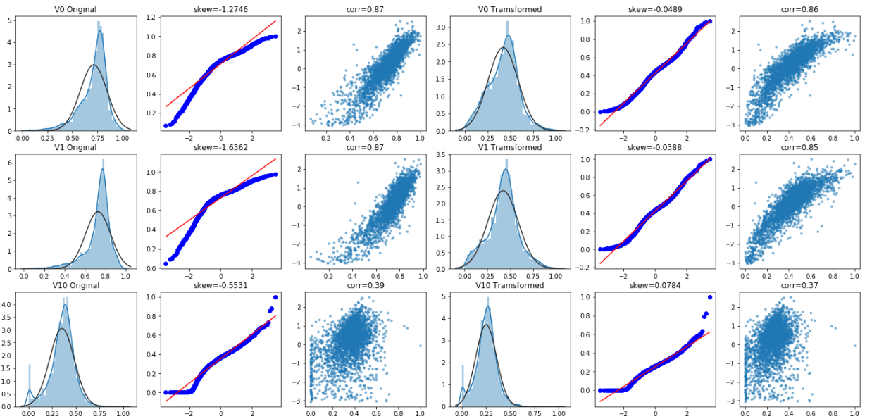
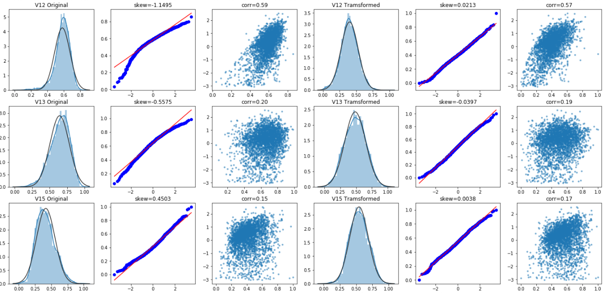
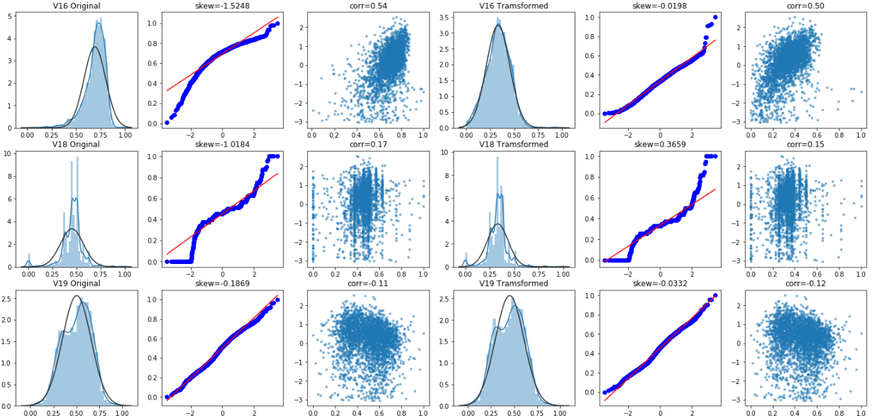
Box Cox transformation
Box Cox transformation is a data transformation commonly used in statistical modeling, which is used when continuous response variables do not meet the normal distribution. For example, when using linear regression, due to the residual ϵ \epsilon ϵ If it does not conform to the normal distribution and does not meet the modeling conditions, the response variable Y should be transformed to turn the data into normal. After box Cox transform, the correlation between residual and prediction variables can be reduced to a certain extent.

# Box Cox transformation
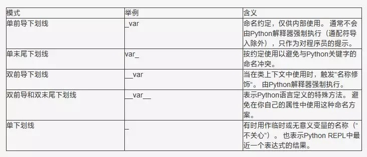
#Meaning of underline in Python: https://www.runoob.com/w3cnote/python-5-underline.html
cols_transform=data_all.columns[0:-2]
for col in cols_transform:   
    # transform column
    #boxcox requires the input data to be positive.
    #stats.boxcox() returns a positive data set converted to the power of box Cox
    data_all.loc[:,col], _ = stats.boxcox(data_all.loc[:,col]+1)

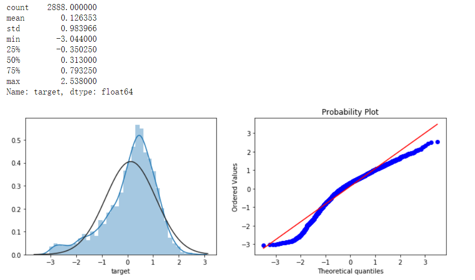
print(data_all.target.describe())
plt.figure(figsize=(12,4))
plt.subplot(1,2,1)
sns.distplot(data_all.target.dropna() , fit=stats.norm)
plt.subplot(1,2,2)
_ = stats.probplot(data_all.target.dropna(), plot=plt)

Meaning of underline in python:

Use logarithmic transformation target value to improve the normality of characteristic data. Refer to: https://www.zhihu.com/question/22012482

sp = data_train.target
data_train.target1 = np.power(1.5,sp)
print(data_train.target1.describe())

plt.figure(figsize=(12,4))
plt.subplot(1,2,1)
sns.distplot(data_train.target1.dropna(),fit=stats.norm)
plt.subplot(1,2,2)
_=stats.probplot(data_train.target1.dropna(), plot=plt)

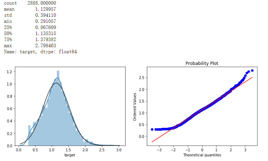
As can be seen from the QQ chart, the normality has been improved.

4. Model building and integrated learning

Build training set and test set

Separate the previously merged training set from the test set, and then delete some attribute values added manually and irrelevant to training

# function to get training samples
def get_training_data():
    # extract training samples
    from sklearn.model_selection import train_test_split
    df_train = data_all[data_all["oringin"]=="train"]
    df_train["label"]=data_train.target1
    # split SalePrice and features
    y = df_train.target
    X = df_train.drop(["oringin","target","label"],axis=1)
    X_train,X_valid,y_train,y_valid=train_test_split(X,y,test_size=0.3,random_state=100)
    return X_train,X_valid,y_train,y_valid

# extract test data (without SalePrice)
def get_test_data():
    df_test = data_all[data_all["oringin"]=="test"].reset_index(drop=True)
    return df_test.drop(["oringin","target"],axis=1)

Evaluation function of rmse and mse

from sklearn.metrics import make_scorer
# metric for evaluation
def rmse(y_true, y_pred):
    diff = y_pred - y_true
    sum_sq = sum(diff**2)    
    n = len(y_pred)   
    return np.sqrt(sum_sq/n)

def mse(y_ture,y_pred):
    return mean_squared_error(y_ture,y_pred)

# scorer to be used in sklearn model fitting
rmse_scorer = make_scorer(rmse, greater_is_better=False) 

#Entered score_ When func is a scoring function, the value is True (default value); This value is False when the input function is a loss function
mse_scorer = make_scorer(mse, greater_is_better=False)

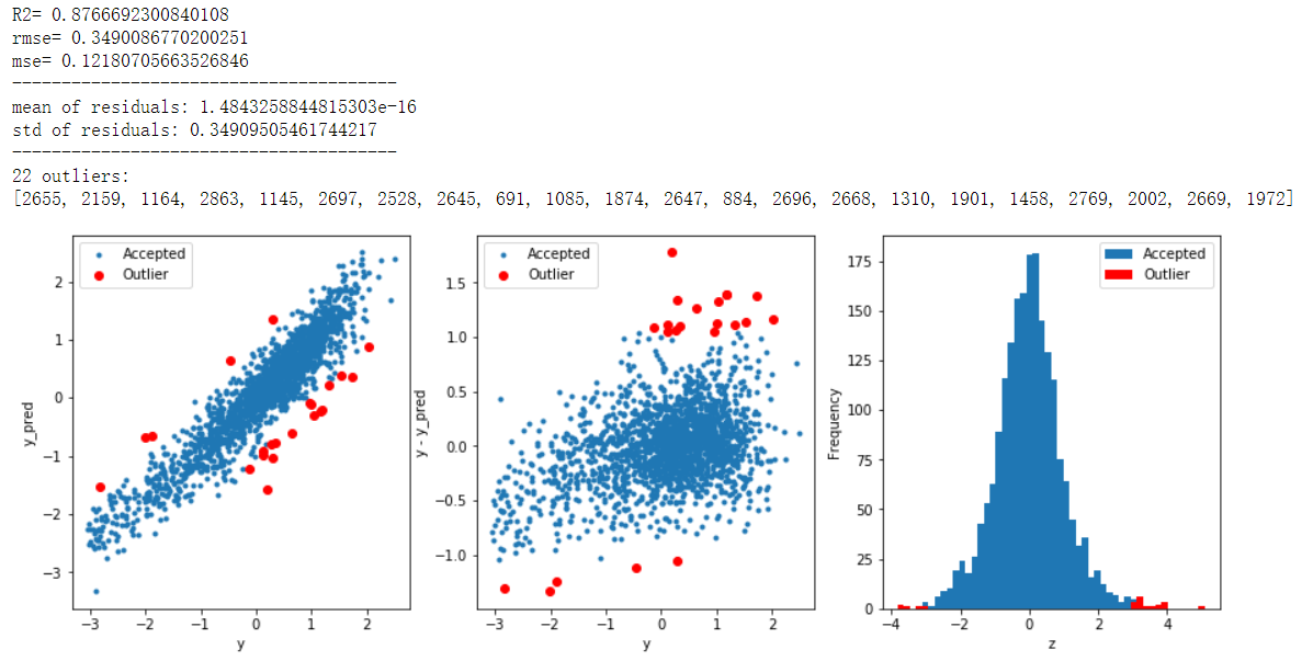
Find outliers and delete

# function to detect outliers based on the predictions of a model
def find_outliers(model, X, y, sigma=3):

    # predict y values using model
    model.fit(X,y)
    y_pred = pd.Series(model.predict(X), index=y.index)
        
    # calculate residuals between the model prediction and true y values
    resid = y - y_pred
    mean_resid = resid.mean()
    std_resid = resid.std()

    # calculate z statistic, define outliers to be where |z|>sigma
    z = (resid - mean_resid)/std_resid    
    outliers = z[abs(z)>sigma].index
    
    # print and plot the results
    print('R2=',model.score(X,y))
    print('rmse=',rmse(y, y_pred))
    print("mse=",mean_squared_error(y,y_pred))
    print('---------------------------------------')

    print('mean of residuals:',mean_resid)
    print('std of residuals:',std_resid)
    print('---------------------------------------')

    print(len(outliers),'outliers:')
    print(outliers.tolist())

    plt.figure(figsize=(15,5))
    ax_131 = plt.subplot(1,3,1)
    plt.plot(y,y_pred,'.')
    plt.plot(y.loc[outliers],y_pred.loc[outliers],'ro')
    plt.legend(['Accepted','Outlier'])
    plt.xlabel('y')
    plt.ylabel('y_pred');

    ax_132=plt.subplot(1,3,2)
    plt.plot(y,y-y_pred,'.')
    plt.plot(y.loc[outliers],y.loc[outliers]-y_pred.loc[outliers],'ro')
    plt.legend(['Accepted','Outlier'])
    plt.xlabel('y')
    plt.ylabel('y - y_pred');

    ax_133=plt.subplot(1,3,3)
    z.plot.hist(bins=50,ax=ax_133)
    z.loc[outliers].plot.hist(color='r',bins=50,ax=ax_133)
    plt.legend(['Accepted','Outlier'])
    plt.xlabel('z')
    
    return outliers

# get training data
X_train, X_valid,y_train,y_valid = get_training_data()
test=get_test_data()

# find and remove outliers using a Ridge model
outliers = find_outliers(Ridge(), X_train, y_train)
X_outliers=X_train.loc[outliers]
y_outliers=y_train.loc[outliers]
X_t=X_train.drop(outliers)
y_t=y_train.drop(outliers)

model training

def get_trainning_data_omitoutliers():
    #Obtain training data and omit outliers
    y=y_t.copy()
    X=X_t.copy()
    return X,y

def train_model(model, param_grid=[], X=[], y=[], 
                splits=5, repeats=5):

    # get data
    if len(y)==0:
        X,y = get_trainning_data_omitoutliers()
        
    # Cross validation
    rkfold = RepeatedKFold(n_splits=splits, n_repeats=repeats)
    
    # Optimal parameters of grid search
    if len(param_grid)>0:
        gsearch = GridSearchCV(model, param_grid, cv=rkfold,
                               scoring="neg_mean_squared_error",
                               verbose=1, return_train_score=True)

        # train
        gsearch.fit(X,y)

        # Best model
        model = gsearch.best_estimator_        
        best_idx = gsearch.best_index_

        # Obtain cross validation evaluation indicators
        grid_results = pd.DataFrame(gsearch.cv_results_)
        cv_mean = abs(grid_results.loc[best_idx,'mean_test_score'])
        cv_std = grid_results.loc[best_idx,'std_test_score']

    # No grid search  
    else:
        grid_results = []
        cv_results = cross_val_score(model, X, y, scoring="neg_mean_squared_error", cv=rkfold)
        cv_mean = abs(np.mean(cv_results))
        cv_std = np.std(cv_results)
    
    # Merge data
    cv_score = pd.Series({'mean':cv_mean,'std':cv_std})

    # forecast
    y_pred = model.predict(X)
    
    # Statistics of model performance        
    print('----------------------')
    print(model)
    print('----------------------')
    print('score=',model.score(X,y))
    print('rmse=',rmse(y, y_pred))
    print('mse=',mse(y, y_pred))
    print('cross_val: mean=',cv_mean,', std=',cv_std)
    
    # Residual analysis and visualization
    y_pred = pd.Series(y_pred,index=y.index)
    resid = y - y_pred
    mean_resid = resid.mean()
    std_resid = resid.std()
    z = (resid - mean_resid)/std_resid    
    n_outliers = sum(abs(z)>3)
    outliers = z[abs(z)>3].index
    
    return model, cv_score, grid_results

# Define training variables to store data
opt_models = dict()
score_models = pd.DataFrame(columns=['mean','std'])
splits=5
repeats=5

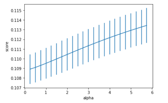
model = 'Ridge'  #Replaceable, see various models in case analysis I
opt_models[model] = Ridge() #Replaceable, see various models in case analysis I
alph_range = np.arange(0.25,6,0.25)
param_grid = {'alpha': alph_range}

opt_models[model],cv_score,grid_results = train_model(opt_models[model], param_grid=param_grid, 
                                              splits=splits, repeats=repeats)

cv_score.name = model
score_models = score_models.append(cv_score)

plt.figure()
plt.errorbar(alph_range, abs(grid_results['mean_test_score']),
             abs(grid_results['std_test_score'])/np.sqrt(splits*repeats))
plt.xlabel('alpha')
plt.ylabel('score')

# Prediction function
def model_predict(test_data,test_y=[]):
    i=0
    y_predict_total=np.zeros((test_data.shape[0],))
    for model in opt_models.keys():
        if model!="LinearSVR" and model!="KNeighbors":
            y_predict=opt_models[model].predict(test_data)
            y_predict_total+=y_predict
            i+=1
        if len(test_y)>0:
            print("{}_mse:".format(model),mean_squared_error(y_predict,test_y))
    y_predict_mean=np.round(y_predict_total/i,6)
    if len(test_y)>0:
        print("mean_mse:",mean_squared_error(y_predict_mean,test_y))
    else:
        y_predict_mean=pd.Series(y_predict_mean)
        return y_predict_mean

#Model prediction and result saving
y_ = model_predict(test)
y_.to_csv('predict.txt',header = None,index = False)