1.Logistic Regression

Given Data X = x 1 , x 2 , . . . , X={x_1,x_2,...,} X=x1​,x2​,...,, Y = y 1 , y 2 , . . . , Y={y_1,y_2,...,} Y=y1, y2,..., Consider a binary task, that is y i ∈ 0 , 1 , i = 1 , 2 , . . . y_i\in{{0,1}},i=1,2,... yi​∈0,1,i=1,2,...,

Hypothesis function

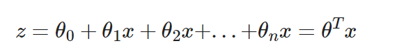
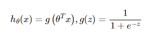
Assume that the function is its basic model, as follows: h θ ( x ) = g ( θ T x ) h_{\theta}(x)=g(\theta^{T}x) h θ (x)=g( θ Tx) where θ T x = w T x + b \theta^{T}x=w^Tx+b θ Tx=wTx+b, and g ( z ) = 1 1 + e − z g(z)=\frac{1}{1+e^{-z}} g(z)=1+e_z1 is s i g m o i d sigmoid The sigmoid function, also known as the activation function.

loss function

Loss function, also known as cost function, is used to measure the quality of a model. Here, a loss function can be defined by the maximum likelihood estimation method.

The difference between likelihood and probability and what is a maximum likelihood estimate. Understand Maximum Likelihood Estimation

The cost function can be defined as a maximum likelihood estimate, i.e. L ( θ ) = ∏ i = 1 p ( y i = 1 ∣ x i ) = h θ ( x 1 ) ( 1 − h θ ( x 2 ) ) . . . L(\theta)=\prod_{i=1}p(y_i=1|x_i)=h_\theta(x_1)(1-h_\theta(x_2))... L( θ)= _i=1 p(yi=1_xi)=h θ (x1) (1_h) θ (x2)..., among x 1 x_1 x1 corresponding label y 1 = 1 y_1=1 y1​=1， x 2 x_2 x2 corresponding label y 2 = 0 y_2=0 y2 = 0, which sets the probability of positive cases to h θ ( x i ) h_\theta(x_i) hθ​(xi​): p ( y i = 1 ∣ x i ) = h θ ( x i ) p(y_i=1|x_i)=h_\theta(x_i) p(yi​=1∣xi​)=hθ​(xi​) p ( y i = 0 ∣ x i ) = 1 − h θ ( x i ) p(y_i=0|x_i)=1-h_\theta(x_i) p(yi​=0∣xi​)=1−hθ​(xi​)

Based on the principle of maximum likelihood estimation, our goal is θ ∗ = arg ⁡ max ⁡ θ L ( θ ) \theta^* = \arg \max _{\theta} L(\theta) θ∗=argθmax​L(θ)

To simplify the operation, add logarithms on both sides to get θ ∗ = arg ⁡ max ⁡ θ L ( θ ) ⇒ θ ∗ = arg ⁡ min ⁡ θ − ln ⁡ ( L ( θ ) ) \theta^* = \arg \max _{\theta} L(\theta) \Rightarrow \theta^* = \arg \min _{\theta} -\ln(L(\theta)) θ∗=argθmax​L(θ)⇒θ∗=argθmin​−ln(L(θ))

Simplified (for code purposes only, reference watermelon book for specific derivation): − ln ⁡ ( L ( θ ) ) = ℓ ( θ ) = ∑ i = 1 ( − y i θ T x i + ln ⁡ ( 1 + e θ T x i ) ) -\ln(L(\theta))=\ell(\boldsymbol{\theta})=\sum_{i=1}(-y_i\theta^Tx_i+\ln(1+e^{\theta^Tx_i})) −ln(L(θ))=ℓ(θ)=i=1∑​(−yi​θTxi​+ln(1+eθTxi​))

Solution: Gradient descent

Based on convex optimization theory, the function can be solved by gradient descent method and Newton method.

For gradient descent, where η \eta η For learning rate: θ t + 1 = θ t − η ∂ ℓ ( θ ) ∂ θ \theta^{t+1}=\theta^{t}-\eta \frac{\partial \ell(\boldsymbol{\theta})}{\partial \boldsymbol{\theta}} θ t+1= θ t_ η _ θ _( θ) Where ∂ ℓ ( θ ) ∂ θ = ∑ i = 1 ( − y i x i + e θ T x i x i 1 + e θ T x i ) = ∑ i = 1 x i ( − y i + h θ ( x i ) ) = ∑ i = 1 x i ( − e r r o r ) \frac{\partial \ell(\boldsymbol{\theta})}{\partial \boldsymbol{\theta}}=\sum_{i=1}(-y_ix_i+\frac{e^{\theta^Tx_i}x_i}{1+e^{\theta^Tx_i}})=\sum_{i=1}x_i(-y_i+h_\theta(x_i))=\sum_{i=1}x_i(-error) ∂θ∂ℓ(θ)​=i=1∑​(−yi​xi​+1+eθTxi​eθTxi​xi​​)=i=1∑​xi​(−yi​+hθ​(xi​))=i=1∑​xi​(−error)

Gradients rise more easily here: θ t + 1 = θ t + η − ∂ ℓ ( θ ) ∂ θ \theta^{t+1}=\theta^{t}+\eta \frac{-\partial \ell(\boldsymbol{\theta})}{\partial \boldsymbol{\theta}} θ t+1= θ t+ η _ θ _( θ) Where − ∂ ℓ ( θ ) ∂ θ = ∑ i = 1 ( y i x i − e θ T x i x i 1 + e θ T x i ) = ∑ i = 1 x i ( y i − h θ ( x i ) ) = ∑ i = 1 x i ∗ e r r o r \frac{-\partial \ell(\boldsymbol{\theta})}{\partial \boldsymbol{\theta}}=\sum_{i=1}(y_ix_i-\frac{e^{\theta^Tx_i}x_i}{1+e^{\theta^Tx_i}})=\sum_{i=1}x_i(y_i-h_\theta(x_i))=\sum_{i=1}x_i*error ∂θ−∂ℓ(θ)​=i=1∑​(yi​xi​−1+eθTxi​eθTxi​xi​​)=i=1∑​xi​(yi​−hθ​(xi​))=i=1∑​xi​∗error

Pseudocode

The training algorithm is as follows:

Input: Training data X = x 1 , x 2 , . . . , x n X={x_1,x_2,...,x_n} X=x1, x2,..., xn, training label Y = y 1 , y 2 , . . . , Y={y_1,y_2,...,} Y=y1, y2,...,, Notice that they are all in matrix form

Output: trained model parameters θ \theta θ， perhaps h θ ( x ) h_{\theta}(x) hθ​(x)

Initialize model parameters θ \theta θ， Number of iterations n i t e r s n_iters ni ters, learning rate η \eta η

$\mathbf{FOR} \ i_iter \ \mathrm{in \ range}(n_iters)$
$\mathbf{FOR} \ i \ \mathrm{in \ range}(n)$   $\rightarrow n=len(X)$
$error=y_i-h_{\theta}(x_i)$
$grad=error*x_i$
$\theta \leftarrow \theta + \eta*grad$   $\rightarrow$Gradient rise
$\mathbf{END \ FOR}$
$\mathbf{END \ FOR}$

regression

Depending on the dependent variable, there are several regressions:

• Continuity: Multiple linear regression (Note that there are differences between multiple linear regression, such as continuous multivariate independent variables, multiple data types, etc.)
• Binomial distribution: logistic regression
• poisson distribution: poisson regression
• Negative binomial distribution: negative binomial regression
• Logistic regression, like linear regression, requires n parameters:
  Logistic regression introduces non-linear factors through the Sigmoid function, which makes it easy to deal with bi-classification problems:
  Unlike linear regression, logistic regression uses the cross-entropy loss function: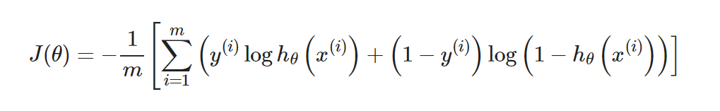Its gradient is:
  
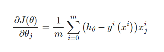
  The form is the same as linear regression, but the hypothesis function is different. Logical regression is: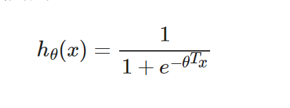

import sys
from pathlib import Path
curr_path = str(Path().absolute())
parent_path = str(Path().absolute().parent)
sys.path.append(parent_path) # add current terminal path to sys.path

import numpy as np
from Mnist.load_data import load_local_mnist

(x_train, y_train), (x_test, y_test) = load_local_mnist(one_hot=False)

# print(np.shape(x_train),np.shape(y_train))

ones_col=[[1] for i in range(len(x_train))] # Generate a two-dimensional nested list of all 1, that is, [[1], [1],..., [1]]
x_train_modified=np.append(x_train,ones_col,axis=1)
ones_col=[[1] for i in range(len(x_test))]
x_test_modified=np.append(x_test,ones_col,axis=1)

# print(np.shape(x_train_modified))

# Mnsit e has 10 tags, so since it's a bi-categorized task, you can use tag 0 as a 1, and the rest as a 0 to identify if it's a 0 task
y_train_modified=np.array([1 if y_train[i]==1 else 0 for i in range(len(y_train))])
y_test_modified=np.array([1 if y_test[i]==1 else 0 for i in range(len(y_test))])
n_iters=10 

x_train_modified_mat = np.mat(x_train_modified)
theta = np.mat(np.zeros(len(x_train_modified[0])))
lr = 0.01 # learning rate

def sigmoid(x):
    '''sigmoid function
    '''
    return 1.0/(1+np.exp(-x)) 

Mini-batch Gradient Descent

for i_iter in range(n_iters):
    for n in range(len(x_train_modified)):
        hypothesis = sigmoid(np.dot(x_train_modified[n], theta.T))
        error = y_train_modified[n]- hypothesis
        grad = error*x_train_modified_mat[n]
        theta += lr*grad
    print('LogisticRegression Model(learning_rate={},i_iter={})'.format(
    lr, i_iter+1))

1. Getting started with linear regression

1.1 Data Generation

Linear regression is a key to machine learning algorithms. In order to get you started more easily and intuitively, simple data generated by man is used here. The idea of generating data is to set up a two-dimensional function (dimension is too high to be drawn on the plane), generate some discrete data points based on this function, and add a little fluctuation, that is, noise, to each data point, and finally see how our algorithm fits or regresses.

import numpy as np
import matplotlib.pyplot as plt 

def true_fun(X): # This is the real function we set up, the ground true model
    return 1.5*X + 0.2

np.random.seed(0) # Set up random seeds
n_samples = 30 # Set the number of sampling data points

'''Generate random data as training set with some noise'''
X_train = np.sort(np.random.rand(n_samples)) 
y_train = (true_fun(X_train) + np.random.randn(n_samples) * 0.05).reshape(n_samples,1)

1.2 Define Model

After generating the data, we can define our algorithm model and import the LinearRegression class directly from the sklearn library. Because linear regression is simple, there are fewer input parameters for this class and no additional settings are required. After defining the model and training it directly, we can get some parameters that we fit.

from sklearn.linear_model import LinearRegression # Import Linear Regression Model
model = LinearRegression() # Define Model
model.fit(X_train[:,np.newaxis], y_train) # Training model
print("Output parameters w: ",model.coef_) # Output model parameter w
print("Output parameters b: ",model.intercept_) # Output parameter b
 Output parameters w:  [[1.4474774]]
Output parameters b:  [0.22557542]

1.3 Model Test and Comparison

You can see that the parameters of the linear regression fit are 1.44 and 0.22, which are very close to the actual 1.5 and 0.2, indicating that the performance of our algorithm is good. Next, we directly select a batch of data tests, and then draw a picture to see the gap between the algorithm model and the actual model.

X_test = np.linspace(0, 1, 100)
plt.plot(X_test, model.predict(X_test[:, np.newaxis]), label="Model")
plt.plot(X_test, true_fun(X_test), label="True function")
plt.scatter(X_train,y_train) # Draw training set points
plt.legend(loc="best")
plt.show()

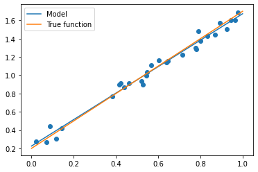
Because our data is relatively simple, we can also see from the graph that our algorithm fits the curve very closely to the actual situation. For more complex and high-dimensional cases, linear regression can not meet our regression needs, so we need to use more advanced polynomial regression.

2. Polynomial Regression

The general idea of polynomial regression is to convert a subpolynomial equation into a linear regression equation, that is, to convert it into a linear regression equation, and then use the linear regression method to find out the corresponding parameters. The same is true for general algorithms. We concatenate the polynomial feature analyzer with the linear regression to calculate the parameters of the linear regression and then push them backwards.

import numpy as np
import matplotlib.pyplot as plt
from sklearn.pipeline import Pipeline
from sklearn.preprocessing import PolynomialFeatures # Import classes that can calculate polynomial characteristics
from sklearn.linear_model import LinearRegression
from sklearn.model_selection import cross_val_score

def true_fun(X): # This is the real function we set up, the ground true model
    return np.cos(1.5 * np.pi * X)
np.random.seed(0)
n_samples = 30 # Set up random seeds

X = np.sort(np.random.rand(n_samples)) 
y = true_fun(X) + np.random.randn(n_samples) * 0.1

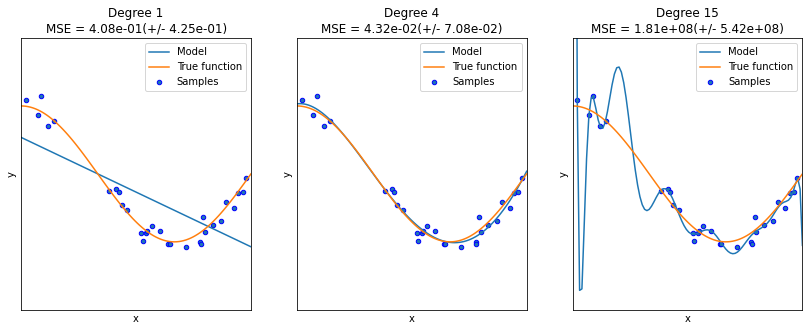
degrees = [1, 4, 15] # Highest degree of polynomial
plt.figure(figsize=(14, 5))
for i in range(len(degrees)):
    ax = plt.subplot(1, len(degrees), i + 1)
    plt.setp(ax, xticks=(), yticks=())
    polynomial_features = PolynomialFeatures(degree=degrees[i],
                                             include_bias=False)
    linear_regression = LinearRegression()
    pipeline = Pipeline([("polynomial_features", polynomial_features),
                         ("linear_regression", linear_regression)]) # Using pipline cascade model
    pipeline.fit(X[:, np.newaxis], y)
    
    scores = cross_val_score(pipeline, X[:, np.newaxis], y,scoring="neg_mean_squared_error", cv=10) # Using cross-validation
    X_test = np.linspace(0, 1, 100)
    plt.plot(X_test, pipeline.predict(X_test[:, np.newaxis]), label="Model")
    plt.plot(X_test, true_fun(X_test), label="True function")
    plt.scatter(X, y, edgecolor='b', s=20, label="Samples")
    plt.xlabel("x")
    plt.ylabel("y")
    plt.xlim((0, 1))
    plt.ylim((-2, 2))
    plt.legend(loc="best")
    plt.title("Degree {}\nMSE = {:.2e}(+/- {:.2e})".format(
        degrees[i], -scores.mean(), scores.std()))
plt.show()

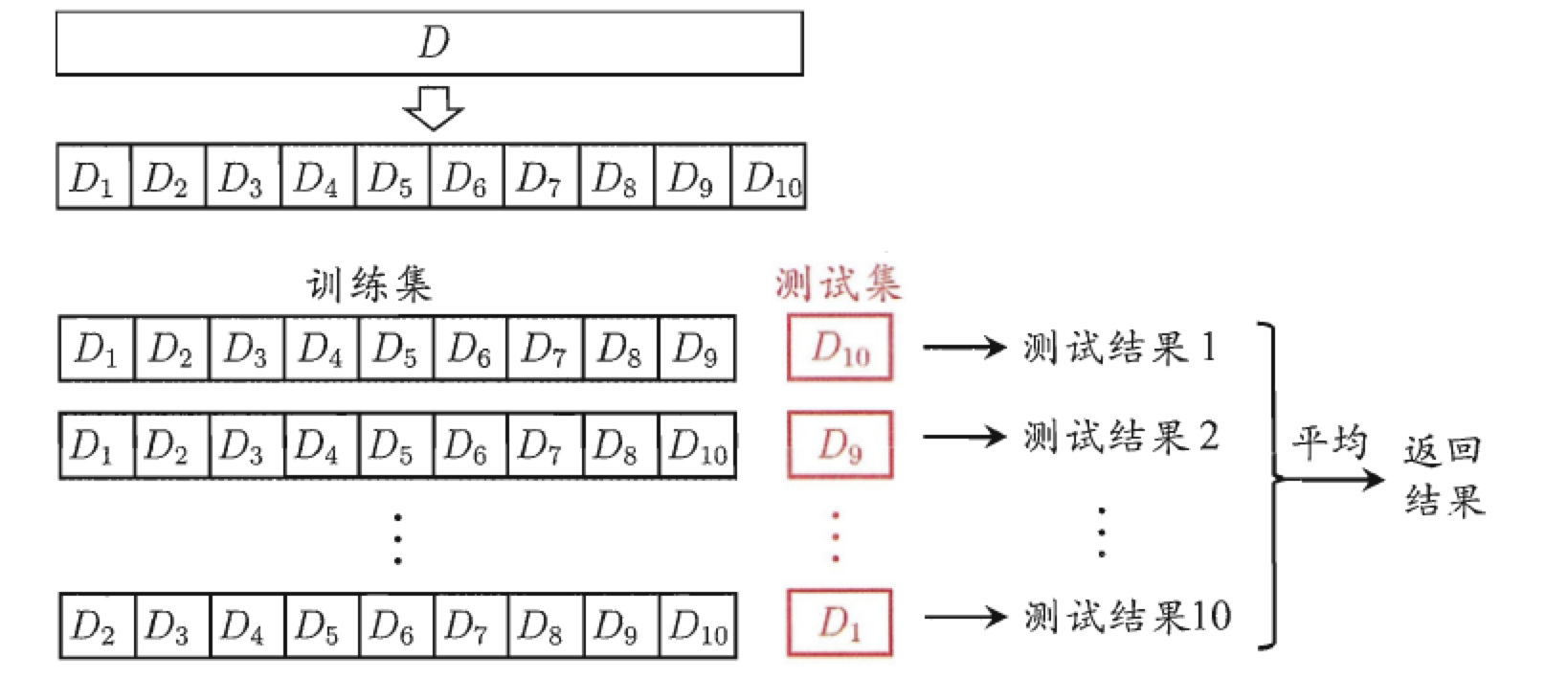
2.1 Cross-validation

One technique we used in this algorithm training is cross-validation. Similar methods include holdout test and self-help (an upgraded version of cross-validation, i.e. the selected data that is put back each time). The purpose of cross-validation is to try to use different training/test set partitions to do different sets of training/tests on the model to cope with the problem of too one-sided test results and insufficient training data. The process is as follows:

2.2 Over-fit and under-fit

We know that polynomial regression may not have different effects on the same data depending on the highest number of times. Higher polynomials can produce more bends to fit more data with non-linear rules, while lower polynomials are close to linear regression. However, in this process, there will also be a problem of over-fitting and under-fitting.