1 Introduction

stay Part I In, we focus on the network structure of DarkNet53 and the structure of YOLOv3, and explain the corresponding detection head
This paper continues the second part of this series, mainly explaining the principle and implementation of YOLO3 model post-processing prediction stage

Don't gossip. Let's start directly 😃

2 understanding output

Before explaining, we need to clarify the following points:

• The input size of YOLOv3 network is (m, 416416,3), where M represents the number of images in each batch. In this explanation, m=1 represents one input image processed by each batch
• YOLOv3 is predicted in three scales, and the size of the characteristic map of the three scales is 13X13,26X26 and 52X52 in turn
• Each cell in YOLOv3 predicts three bounding boxes, and each bounding box can be expressed as 6 tuples ( t x , t y , t w , t h , p c , c ) (t_x,t_y,t_w,t_h,p_c,c) (tx​,ty​,tw​,th​,pc​,c).
• There are 80 categories in the COCO dataset. At this time, we expand c into an 80 dimensional vector, so that each bounding box can be represented by an 85 dimensional vector

Let's take a picture to further elaborate:

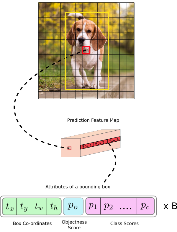
As shown in the figure above:

• The size of the input image is 416X416, down sampled 32 times, and the size of the feature image is 13X13. That is, we divide the input image into 13X13 grids, and each cell corresponds to the 32X32 area in the input image
• If each cell contains the center point of the real frame of the object in the original figure, the cell is responsible for predicting the target. In the above figure, the yellow box is the true value box of the target dog, and the red cell is responsible for predicting the target

3 understand the bounding box

In the YOLOv3 network structure, three branches (three characteristic graphs with different scales) are sent to the decode function for further analysis

In the above figure, the black dashed box represents the priority box (anchor) and the blue solid box represents the prediction box

• b x b_x bx​ b y b_y by​ b w b_w bw​ b h b_h bh ， represents the center point, width and height of our prediction frame
• t x t_x tx​ t y t_y ty​ t w t_w tw​ t h t_h th represents the output of our network
• t x t_x tx​ t y t_y ty represents the offset of the predicted target center relative to the upper left corner coordinate of the cell
• p w p_w pw​ p h p_h ph indicates the width and height of the priority box (anchor)
• c x c_x cx​ c y c_y cy represents the upper left corner coordinate of the cell where the target center is located

Based on the above formula, we can write the corresponding decode function. The relevant explanations have been annotated in the code and will not be repeated

The code implementation is as follows:

def decode(conv_layer,i=0):
	"""
    param: conv_layer nXhXwX255
    """
    n,h,w,c = conv_layer.shape
    conv_output = conv_layer.view(n,h,w,3,5+self.num_class)
    # divide output
    conv_raw_dxdy = conv_output[:, :, :, :, 0:2]  # offset of center position
    conv_raw_dwdh = conv_output[:, :, :, :, 2:4]  # Prediction box length and width offset
    conv_raw_conf = conv_output[:, :, :, :, 4:5]  # confidence of the prediction box
    conv_raw_prob = conv_output[:, :, :, :, 5:]   # category probability of the prediction box

    # grid to 13X13 26X26 52X52
    yv, xv = torch.meshgrid(torch.arange(0, h), torch.arange(0, w))
    yv_new = yv.unsqueeze(dim=-1)
    xv_new = xv.unsqueeze(dim=-1)
    xy_grid = torch.concat([xv_new,yv_new],dim=-1)
    # reshape and repeat
    xy_grid = xy_grid.view(1,h,w,1,2)         # (13,13,2)-->(1,13,13,1,2)
    xy_grid = xy_grid.repeat(n,1,1,3,1).float() # (1,13,13,1,2)--> (1,13,13,3,2)

    # Calculate teh center position  and h&w of the prediction box
    pred_xy = (torch.sigmoid(conv_raw_dxdy) + xy_grid)* self.strides[i]
    pred_wh = (torch.exp(conv_raw_dwdh) * self.anchors[i]) * self.strides[i]
    pred_xywh = torch.concat([pred_xy,pred_wh],dim=-1)
    # score and cls
    pred_conf = torch.sigmoid(conv_raw_conf)
    pred_prob = torch.sigmoid(conv_raw_prob)

    return torch.concat([pred_xywh,pred_conf,pred_prob],dim=-1)

4 NMS post-processing

stay Previous blog The detailed process of NMS has been explained in, and its core idea is briefly summarized as follows:

• Select the box with the highest confidence from the candidate box
• Calculate the IOU of the current box and other boxes, if IOU > IOU_ Threshold removes the corresponding box
• Repeat the above steps to iterate until there are no boxes in the remaining boxes that overlap the currently selected box, iou greater than the threshold

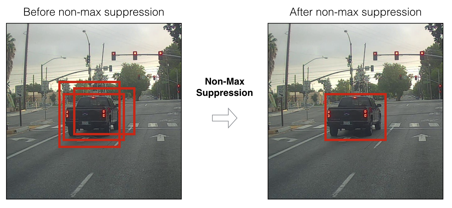
The above process is mainly to filter the box with a large overlap with the current box. For each target, only the box with the highest network prediction confidence is retained. Refer to the following figure:

The code implementation of non maximum suppression is as follows:

def nms(bboxes, iou_threshold, sigma=0.3, method='nms'):
    """
    :param bboxes: (xmin, ymin, xmax, ymax, score, class)
    Note: soft-nms, https://arxiv.org/pdf/1704.04503.pdf
          https://github.com/bharatsingh430/soft-nms
    """
    classes_in_img = list(set(bboxes[:, 5]))
    best_bboxes = []

    for cls in classes_in_img:
        cls_mask = (bboxes[:, 5] == cls)
        cls_bboxes = bboxes[cls_mask]
        # Process 1: Determine whether the number of bounding boxes is greater than 0
        while len(cls_bboxes) > 0:
            # Process 2: Select the bounding box with the highest score according to socre order A
            max_ind = np.argmax(cls_bboxes[:, 4])
            best_bbox = cls_bboxes[max_ind]
            best_bboxes.append(best_bbox)
            cls_bboxes = np.concatenate([cls_bboxes[: max_ind], cls_bboxes[max_ind + 1:]])
            # Process 3: Calculate this bounding box A and
            # Remain all iou of the bounding box and remove those bounding boxes whose iou value is higher than the threshold
            iou = bboxes_iou(best_bbox[np.newaxis, :4], cls_bboxes[:, :4])
            weight = np.ones((len(iou),), dtype=np.float32)

            assert method in ['nms', 'soft-nms']

            if method == 'nms':
                iou_mask = iou > iou_threshold
                weight[iou_mask] = 0.0

            if method == 'soft-nms':
                weight = np.exp(-(1.0 * iou ** 2 / sigma))

            cls_bboxes[:, 4] = cls_bboxes[:, 4] * weight
            score_mask = cls_bboxes[:, 4] > 0.
            cls_bboxes = cls_bboxes[score_mask]

5 load training parameters

In order to run this prediction code, let's load the weight of YOLO3 in official training,

First download the corresponding weight file, as shown below:

wget https://pjreddie.com/media/files/yolov3.weights

Next, let's analyze the official weight file architecture of YOLOv3:

• The official weight file is a binary file, which contains the weights stored in serial mode. The weights are only stored as floating-point numbers, and there is nothing to guide us to which layer they belong
• The weights of YOLOv3 only belong to two types of network layers, one is BN layer and the other is convolution layer. The weights of these layers are stored completely according to the order in which they appear in the configuration file. When BN layer appears in convolution block, convolution does not take bias. When there is no BN layer behind the convolution layer, the convolution takes bias

With the above understanding, let's write the corresponding loading function as follows:

def read_param_from_file(yolo_ckpt,model):
    wf = open(yolo_ckpt, 'rb')
    major, minor, vision, seen, _ = np.fromfile(wf, dtype=np.int32, count=5)
    print("version major={} minor={} vision={} and pic_seen={}".format(major, minor, vision, seen))

    model_dict = model.state_dict()
    key_list = [key for key in model_dict.keys() ]
    num = 6
    length = int(len(key_list)//num)
    pre_index = 0
    for i in range(length+2):
        cur_list = key_list[pre_index:pre_index+num]
        conv_name = cur_list[0]
        conv_layer = model_dict[conv_name]
        filters = conv_layer.shape[0]
        in_dim = conv_layer.shape[1]
        k_size = conv_layer.shape[2]
        conv_shape = (filters,in_dim,k_size,k_size)
        # print("i={} and list={} amd conv_name={} and shape={}".format(i, cur_list,conv_name,conv_shape))
        if len(cur_list) == 6: # with bn
            # darknet bn param:[bias,weight,mean,variance]
            bn_bias = np.fromfile(wf, dtype=np.float32, count= filters)
            model_dict[cur_list[2]].data.copy_( torch.from_numpy(bn_bias))
            bn_weight = np.fromfile(wf, dtype=np.float32, count=filters)
            model_dict[cur_list[1]].data.copy_(torch.from_numpy(bn_weight))
            bn_mean = np.fromfile(wf, dtype=np.float32, count=filters)
            model_dict[cur_list[3]].data.copy_(torch.from_numpy(bn_mean))
            bn_variance = np.fromfile(wf, dtype=np.float32, count=filters)
            model_dict[cur_list[4]].data.copy_(torch.from_numpy(bn_variance))
            # darknet conv param:(out_dim, in_dim, height, width)
            conv_weights = np.fromfile(wf, dtype=np.float32, count=np.product(conv_shape))
            conv_weights = conv_weights.reshape(conv_shape)
            model_dict[cur_list[0]].data.copy_(torch.from_numpy(conv_weights))
        else:
            conv_bias = np.fromfile(wf, dtype=np.float32, count= filters)
            model_dict[cur_list[1]].data.copy_(torch.from_numpy(conv_bias))
            conv_weights = np.fromfile(wf, dtype=np.float32, count=np.product(conv_shape))
            conv_weights = conv_weights.reshape(conv_shape)
            model_dict[cur_list[0]].data.copy_(torch.from_numpy(conv_weights))

        pre_index += num
        if i in [57, 65, 73]:
            num = 2
        else:
            num = 6
    assert len(wf.read()) == 0, 'failed to read all data'

6 final effect

Code cloning:

git clone git@github.com:sgzqc/yolov3_pytorch.git

Run script:

python3 LoadModel.py

The results are as follows:

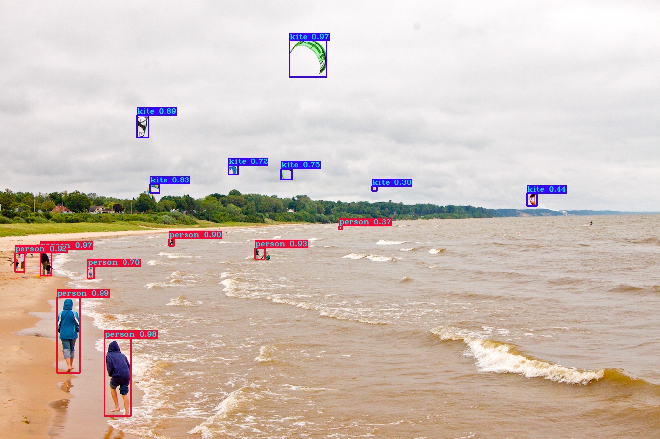
Output at IOU threshold 0.3:

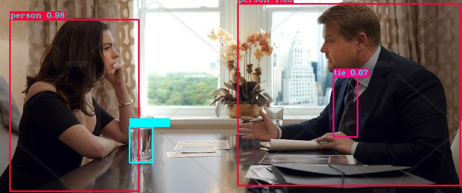
Output at IOU threshold 0.5:

7 Summary

This section mainly explains the reasoning decoding part and network post-processing part of YOLO v3 network, focusing on the decoding of prediction header and the code implementation of NMS in post-processing, and gives a complete code link

Have you failed?

Pay attention to the official account, and then reply to yolov3, then you can get the complete code link.

Pay attention to the official account of AI algorithm and get more AI algorithm information.