Technical dry goods | better understanding of Focal Loss based on mindspire

Posted by CBR on Fri, 04 Mar 2022 00:35:10 +0100

Abstract: Focal Loss is a loss function proposed by Kaiming great God team in their paper Focal Loss for sense object detection. It is used to improve the effect of image object detection.

This article is shared from Huawei cloud community< Technical dry goods | better understanding of Focal Loss based on mindspire >, original author: chengxiaoli.

Today, we update the Focal Loss of Kaiming great God, which is the loss function proposed by Kaiming great God team in their paper Focal Loss for Dense Object Detection. It is used to improve the effect of image object detection. ICCV2017RBG and Kaiming's new work( https://arxiv.org/pdf/1708.02002.pdf ).

Usage scenario

Recently, we have been working on the direction related to facial expression. The number of datasets in this field is small, and there is often the problem of imbalance between positive and negative samples. Generally speaking, there are two ways to solve the problem of unbalanced number of positive and negative samples:

1. Design sampling strategy, generally resampling a small number of samples

2. The design of Loss is generally to assign weights to samples of different categories

I have used both strategies. This article is about Focal Loss in the second strategy.

Thesis analysis

We know that object detection is generally divided into two categories according to its process. One is the two stage detector (such as the classic fast r-cnn and RFCN, which need the detection algorithm of region proposal), and the second is the one stage detector (such as SSD and YOLO series, which do not need the detection algorithm of region proposal and direct regression).

For the first kind of algorithm, it can achieve high accuracy, but the speed is slow. Although the speed can be increased by reducing the number of proposal s or reducing the resolution of the input image, the speed has not been qualitatively improved.

For the second kind of algorithm, the speed is very fast, but the accuracy is not as good as the first kind.

So the goal is: the starting point of focal loss is to hope that one stage detector can achieve the accuracy of two stage detector without affecting the original speed.

So，Why？and result？

What causes this? the Reason is: class imbalance.

We know that in the field of object detection, an image may generate thousands of candidate locations, but only a few of them contain objects, which leads to category imbalance. So what are the consequences of category imbalance? Two consequences of quoting the original text:

(1) training is inefficient as most locations are easy negatives that contribute no useful learning signal;
(2) en masse, the easy negatives can overwhelm training and lead to degenerate models.

It means that the number of negative samples is too large (belonging to background samples), accounting for most of the total loss, and most of them are easy to classify, so the optimization direction of the model is not what we want. In this way, the network can not learn useful information and can not accurately classify object s. In fact, there are some previous algorithms to deal with the problem of category imbalance, such as OHEM (online hard example mining). The main idea of OHEM can be summarized in one sentence of the original text: in OHEM each example is scored by its loss, non maximum suppression (NMS) is then applied, and a minimum is constructed with the highest loss examples. Although OHEM algorithm increases the weight of misclassified samples, OHEM algorithm ignores the samples that are easy to classify.

Therefore, aiming at the problem of category imbalance, the author proposes a new loss function: Focal Loss, which is modified based on the standard cross entropy loss. It is easier to focus on the classification of samples through the training function, which can reduce the weight of samples. In order to prove the effectiveness of Focal Loss, the author designed a deny detector: RetinaNet, and used Focal Loss training in training. Experiments show that RetinaNet can not only achieve the speed of one stage detector, but also have the accuracy of two stage detector.

Formula description

Introduce focal loss. Before introducing focal loss, let's take a look at the loss of cross entropy. Here, take the second classification as an example. The original classification loss is the direct summation of the cross entropy of each training sample, that is, the weight of each sample is the same. The formula is as follows:

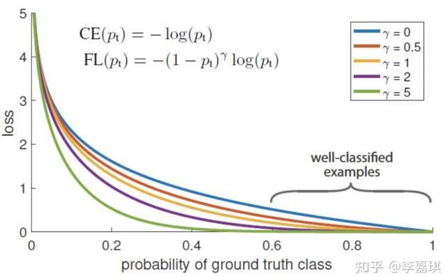
Because it is a binary classification, P represents the probability that the prediction sample belongs to 1 (the range is 0-1), Y represents label, and the value of Y is {+ 1, - 1}. When the real label is 1, that is, y=1, if the probability p of a sample x is predicted to be 1 is 0.6, then the loss is - log(0.6). Note that the loss is greater than or equal to 0. If p=0.9, the loss is - log(0.9), so the loss of p=0.6 is greater than that of p=0.9, which is easy to understand. Here, we only take the two classification as an example, and the multi classification as an analogy. For convenience, pt is used instead of P, as shown in formula 2:. pt here is the abscissa in Figure 1.

For simplicity, we use p_t indicates the probability that the sample belongs to true class. Therefore, equation (1) can be written as:

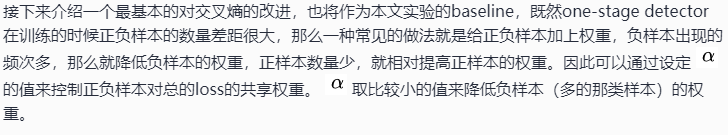
Obviously, although the previous formula 3 can control the weight of positive and negative samples, it can not control the weight of easy and difficult samples, so there is Focal Loss γ Called focusing parameter, γ>= 0, called modulation coefficient:

Why add this modulation coefficient? The purpose is to reduce the weight of easy to classify samples, so as to make the model focus on difficult to classify samples during training.

Through the experiment, it is found that the drawing is shown in Figure 1 below. The abscissa is pt and the ordinate is loss. CE (pt) represents the standard cross entropy formula, and FL (pt) represents the improved cross entropy used in focal loss. In Figure 1 γ= The blue curve of 0 is the standard cross entropy loss.

This not only solves the imbalance between positive and negative samples, but also solves the imbalance between easy and hard samples.

conclusion

The author takes category imbalance as the main reason that hinders the one stage method from surpassing the top performing two stage method. In order to solve this problem, the author proposes focal loss, which uses an adjustment item in the cross entropy, in order to focus the learning on hard examples and reduce the weight of a large number of easy negatives. It solves the imbalance between positive and negative samples and the problem of distinguishing simple and complex samples at the same time.

Let's take a look at the code to realize Focal Loss based on mindspire:

import mindspore
import mindspore.common.dtype as mstype
from mindspore.common.tensor import Tensor
from mindspore.common.parameter import Parameter
from mindspore.ops import operations as P
from mindspore.ops import functional as F
from mindspore import nn

class FocalLoss(_Loss):

    def __init__(self, weight=None, gamma=2.0, reduction='mean'):
        super(FocalLoss, self).__init__(reduction=reduction)
        # Check gamma, here γ Called focusing parameter, γ>= 0, called modulation coefficient
        self.gamma = validator.check_value_type("gamma", gamma, [float])
        if weight is not None and not isinstance(weight, Tensor):
            raise TypeError("The type of weight should be Tensor, but got {}.".format(type(weight)))
        self.weight = weight
        # Mindscore operator used
        self.expand_dims = P.ExpandDims()
        self.gather_d = P.GatherD()
        self.squeeze = P.Squeeze(axis=1)
        self.tile = P.Tile()
        self.cast = P.Cast()

    def construct(self, predict, target):
        targets = target
        # Verify the input
        _check_ndim(predict.ndim, targets.ndim)
        _check_channel_and_shape(targets.shape[1], predict.shape[1])
        _check_predict_channel(predict.shape[1])

        # Change the shapes of logits and target to num_batch * num_class * num_voxels.
        if predict.ndim > 2:
            predict = predict.view(predict.shape[0], predict.shape[1], -1) # N,C,H,W => N,C,H*W
            targets = targets.view(targets.shape[0], targets.shape[1], -1) # N,1,H,W => N,1,H*W or N,C,H*W
        else:
            predict = self.expand_dims(predict, 2) # N,C => N,C,1
            targets = self.expand_dims(targets, 2) # N,1 => N,1,1 or N,C,1
 
        # Calculate logarithmic probability
        log_probability = nn.LogSoftmax(1)(predict)
        # Only the logarithmic probability value of the ground truth class of each voxel is retained.
        if target.shape[1] == 1:
            log_probability = self.gather_d(log_probability, 1, self.cast(targets, mindspore.int32))
            log_probability = self.squeeze(log_probability)

        # Get probability
        probability = F.exp(log_probability)

        if self.weight is not None:
            convert_weight = self.weight[None, :, None]  # C => 1,C,1
            convert_weight = self.tile(convert_weight, (targets.shape[0], 1, targets.shape[2])) # 1,C,1 => N,C,H*W
            if target.shape[1] == 1:
                convert_weight = self.gather_d(convert_weight, 1, self.cast(targets, mindspore.int32))  # selection of the weights  => N,1,H*W
                convert_weight = self.squeeze(convert_weight)  # N,1,H*W => N,H*W
            # Multiply the logarithmic probabilities by their weights
            probability = log_probability * convert_weight
        # Calculate the loss of small batch
        weight = F.pows(-probability + 1.0, self.gamma)
        if target.shape[1] == 1:
            loss = (-weight * log_probability).mean(axis=1)  # N
        else:
            loss = (-weight * targets * log_probability).mean(axis=-1)  # N,C

        return self.get_loss(loss)

The usage is as follows:

from mindspore.common import dtype as mstype
from mindspore import nn
from mindspore import Tensor

predict = Tensor([[0.8, 1.4], [0.5, 0.9], [1.2, 0.9]], mstype.float32)
target = Tensor([[1], [1], [0]], mstype.int32)
focalloss = nn.FocalLoss(weight=Tensor([1, 2]), gamma=2.0, reduction='mean')
output = focalloss(predict, target)
print(output)

0.33365273

Two important properties of Focal Loss

1. When a sample is wrongly divided and Pt is very small, the modulation factor (1-Pt) is close to 1 and the loss is not affected; When Pt → 1 and the factor (1-Pt) is close to 0, the weight of the well classified sample will be lowered. Therefore, the modulation coefficient tends to 1, that is, there is no big change compared with the original loss. When Pt tends to 1 (at this time, the classification is correct and it is easy to classify samples), the modulation coefficient tends to 0, that is, the contribution to the total loss is very small.

2. When γ= When the loss of entropy is 0, the loss of entropy is 0 γ When it increases, the modulation coefficient will also increase. Focus parameter γ The proportion of reducing the weight of easy to divide samples is smoothly adjusted. γ Increasing the modulation factor can enhance the effect of modulation factor γ 2 is the best. Intuitively, the modulation factor reduces the loss contribution of easily divided samples and widens the range of low loss received by samples. When γ At a certain time, for example, equal to 2, the loss of the same easy example(pt=0.9) is 100 + times smaller than the standard cross entropy loss. When pt=0.968, it is 1000 + times smaller, but for hard example (PT < 0.5), the loss is up to 4 times smaller. In this way, the weight of hard example is much higher. This increases the importance of misclassification. The two properties of focal loss are the core. In fact, it is to use an appropriate function to measure the contribution of difficult and easy to classify samples to the total loss.