This article is shared from Huawei cloud community< Keras deep learning Chinese text classification ten thousand word summary (CNN, TextCNN, BiLSTM, attention) >, by eastmount.
I Text classification overview
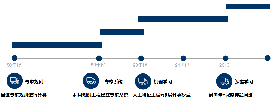
Text classification aims to automatically classify and mark the text set according to a certain classification system or standard. It belongs to an automatic classification based on the classification system. Text classification can be traced back to the 1950s, when text classification was mainly carried out through expert defined rules; In the 1980s, the expert system established by knowledge engineering appeared; In the 1990s, text classification was carried out through artificial feature engineering and shallow classification model with the help of machine learning method. At present, word vector and deep neural network are mostly used for text classification.
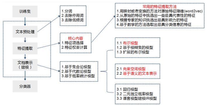
Teacher Niu Yafeng summarized the traditional text classification process as shown in the figure below. In the traditional text classification, most machine learning methods are basically applied in the field of text classification. It mainly includes:
- Naive Bayes
- KNN
- SVM
- Collection class method
- Maximum entropy
- neural network
The basic process of text classification using Keras framework is as follows:
- Step 1: text preprocessing, word segmentation - > remove stop words - > statistics, select top n words as feature words
- Step 2: generate ID for each feature word
- Step 3: convert the text into ID sequence and fill the left
- Step 4: training set shuffle
- Step 5: Embedding Layer converts words into word vectors
- Step 6: add the model and construct the neural network structure
- Step 7: Training Model
- Step 8: get the accuracy, recall and F1 value
Note that if TFIDF is used instead of word vector for document representation, the TFIDF matrix is generated after word segmentation and stop, and then the model is input.
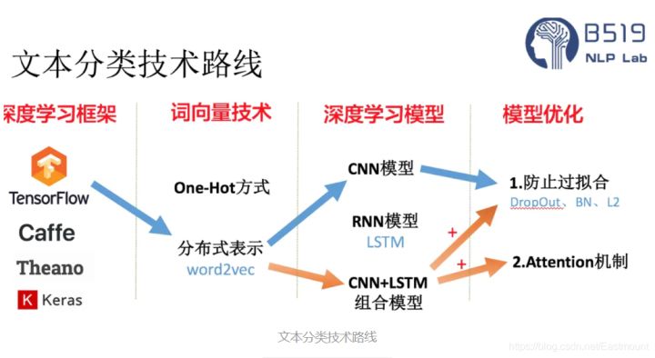
Deep learning text classification methods include:
- Convolutional neural network (TextCNN)
- Cyclic neural network (TextRNN)
- TextRNN+Attention
- TextRCNN(TextRNN+CNN)
- BiLSTM+Attention
- Transfer learning
Recommend teacher Niu Yafeng's article:
- Text classification based on word2vec and CNN: Review & Practice
II Data preprocessing and word segmentation
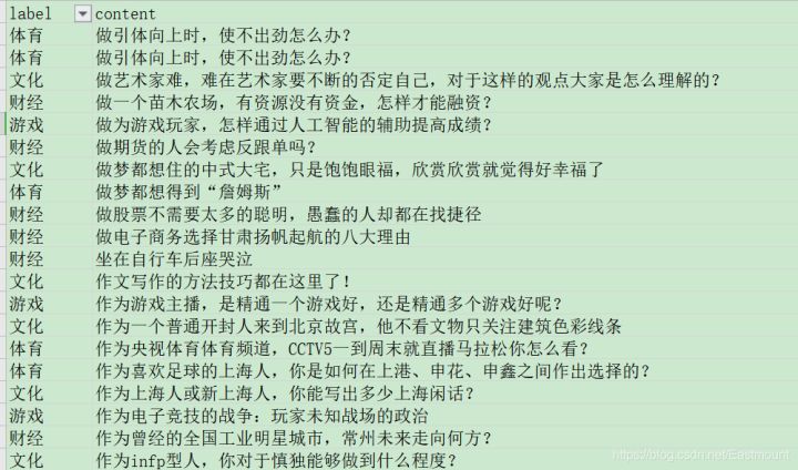
This article mainly focuses on the code, and the algorithm principle knowledge will be supplemented by the previous articles and subsequent articles. The data set is shown in the following figure:
- Training set: news_dataset_train.csv
Game theme (10000), sports theme (10000), cultural theme (10000), financial theme (10000) - Test set: news_dataset_test.csv
Game theme (5000), sports theme (5000), cultural theme (5000), financial theme (5000) - Validation set: news_dataset_val.csv
Game theme (5000), sports theme (5000), cultural theme (5000), financial theme (5000)
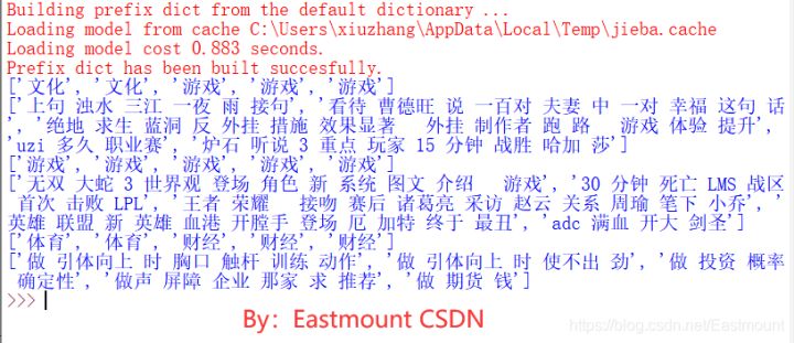
First, we need to preprocess Chinese word segmentation and call Jieba library. The code is as follows:
- data_preprocess.py
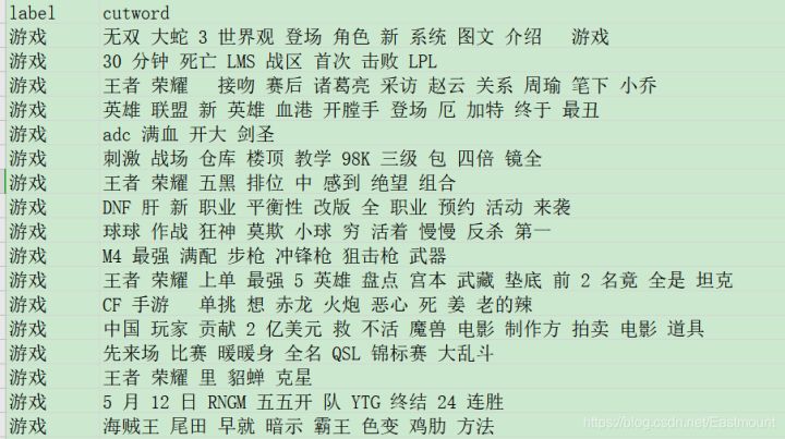
# -*- coding:utf-8 -*-
# By:Eastmount CSDN 2021-03-19
import csv
import pandas as pd
import numpy as np
import jieba
import jieba.analyse

#Add custom dictionaries and deactivate Dictionaries
jieba.load_userdict("user_dict.txt")
stop_list = pd.read_csv('stop_words.txt',
                        engine='python',
                        encoding='utf-8',
                        delimiter="\n",
                        names=['t'])['t'].tolist()

#-----------------------------------------------------------------------
#Jieba word segmentation function
def txt_cut(juzi):
    return [w for w in jieba.lcut(juzi) if w not in stop_list]

#-----------------------------------------------------------------------
#Chinese word segmentation reading file
def fenci(filename,result):
    #Write word segmentation results
    fw = open(result, "w", newline = '',encoding = 'gb18030')
    writer = csv.writer(fw)
    writer.writerow(['label','cutword'])

    #Using CSV Dictreader reads the information in the file
    labels = []
    contents = []
    with open(filename, "r", encoding="UTF-8") as f:
        reader = csv.DictReader(f)
        for row in reader:
            #Data element acquisition
            labels.append(row['label'])
            content = row['content']
            #Chinese word segmentation
            seglist = txt_cut(content)
            #Space splicing
            output = ' '.join(list(seglist))
            contents.append(output)

            #File write
            tlist = []
            tlist.append(row['label'])
            tlist.append(output)
            writer.writerow(tlist)
    print(labels[:5])
    print(contents[:5])
    fw.close()

#-----------------------------------------------------------------------
#Main function
if __name__ == '__main__':
    fenci("news_dataset_train.csv", "news_dataset_train_fc.csv")
    fenci("news_dataset_test.csv", "news_dataset_test_fc.csv")
    fenci("news_dataset_val.csv", "news_dataset_val_fc.csv")
The operation results are shown in the figure below:
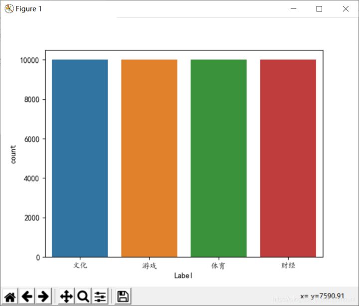
Then we try to simply view the length distribution of data and label visualization.
- data_show.py
# -*- coding: utf-8 -*-
"""
Created on 2021-03-19
@author: xiuzhang Eastmount CSDN
"""
import pandas as pd
import numpy as np
from sklearn import metrics
import matplotlib.pyplot as plt
import seaborn as sns

#---------------------------------------Step 1 data reading------------------------------------
## Read test data set
train_df = pd.read_csv("news_dataset_train_fc.csv")
val_df = pd.read_csv("news_dataset_val_fc.csv")
test_df = pd.read_csv("news_dataset_test_fc.csv")
print(train_df.head())

## Solve the problem of Chinese display
plt.rcParams['font.sans-serif'] = ['KaiTi']  #Specifies the default font SimHei bold
plt.rcParams['axes.unicode_minus'] = False   #Solution: the saved image is a negative sign'

## See which tags are included in the training set
plt.figure()
sns.countplot(train_df.label)
plt.xlabel('Label',size = 10)
plt.xticks(size = 10)
plt.show()

## Analyze the distribution of the number of phrases in the training set
print(train_df.cutwordnum.describe())
plt.figure()
plt.hist(train_df.cutwordnum,bins=100)
plt.xlabel("Phrase length", size = 12)
plt.ylabel("frequency", size = 12)
plt.title("Training data set")
plt.show()
The output results are shown in the figure below. In the following article, we will introduce how to draw good-looking charts.
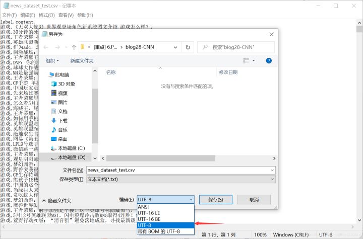
Note that if the error "Unicode decodeerror: 'UTF-8' codec can't decode byte 0xce in position 17: invalid continuation byte" is reported, the CSV file needs to be saved in UTF-8 format, as shown in the following figure.
III CNN Chinese text classification
1. Principle introduction
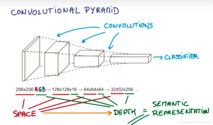
Convolutional neural networks (CNN) is a kind of Feedforward Neural Networks with depth structure including convolution calculation. It is one of the representative algorithms of deep learning. It is usually used in the fields of image recognition and speech recognition, and can give better results. It can also be used in the fields of video analysis, machine translation, natural language processing, drug discovery and so on. The famous alpha dog makes the computer understand that go is based on convolutional neural network.
- Convolution refers to not processing each pixel, but processing the image area. This method strengthens the continuity of the image, sees a graph rather than a point, and also deepens the understanding of the image by the neural network.
- Usually, the convolution neural network will go through the process of "picture - > convolution - > persistence - > convolution - > persistence - > results are transmitted to two fully connected neural layers - > Classifier", and finally realize the classification processing of a CNN.
2. Code implementation
The CNN code of Keras for text classification is as follows:
- Keras_CNN_cnews.py
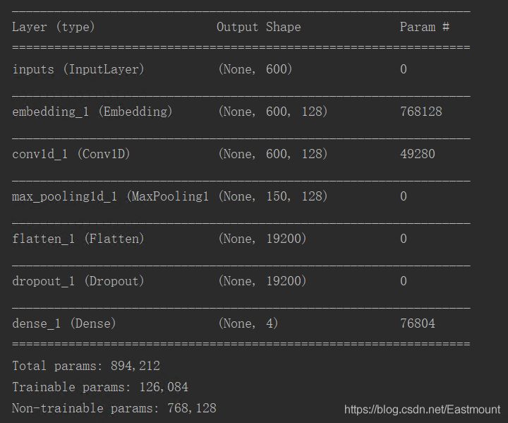
# -*- coding: utf-8 -*-

"""
Created on 2021-03-19
@author: xiuzhang Eastmount CSDN
CNN Model
"""
import os
import time
import pickle
import pandas as pd
import numpy as np
from sklearn import metrics
import matplotlib.pyplot as plt
import seaborn as sns
import tensorflow as tf
from sklearn.preprocessing import LabelEncoder,OneHotEncoder
from keras.models import Model
from keras.layers import LSTM, Activation, Dense, Dropout, Input, Embedding
from keras.layers import Convolution1D, MaxPool1D, Flatten
from keras.preprocessing.text import Tokenizer
from keras.preprocessing import sequence
from keras.callbacks import EarlyStopping
from keras.models import load_model
from keras.models import Sequential

## If the GPU processing reader is a CPU, you can comment on this part of the code
## Specifies the maximum amount of video memory used in each GPU process 0.9 Indicates that it can be used GPU 90%Training with resources
os.environ["CUDA_DEVICES_ORDER"] = "PCI_BUS_IS"
os.environ["CUDA_VISIBLE_DEVICES"] = "0"
gpu_options = tf.GPUOptions(per_process_gpu_memory_fraction=0.8)
sess = tf.Session(config=tf.ConfigProto(gpu_options=gpu_options))

start = time.clock()

#----------------------------Step 1 data reading----------------------------
## Read test data set
train_df = pd.read_csv("news_dataset_train_fc.csv")
val_df = pd.read_csv("news_dataset_val_fc.csv")
test_df = pd.read_csv("news_dataset_test_fc.csv")
print(train_df.head())

## Solve the problem of Chinese display
plt.rcParams['font.sans-serif'] = ['KaiTi']  #Specifies the default font SimHei bold
plt.rcParams['axes.unicode_minus'] = False   #Solution: the saved image is a negative sign'

#--------------------------Step 2 OneHotEncoder()code--------------------
## Encode the label data of the dataset
train_y = train_df.label
val_y = val_df.label
test_y = test_df.label
print("Label:")
print(train_y[:10])

le = LabelEncoder()
train_y = le.fit_transform(train_y).reshape(-1,1)
val_y = le.transform(val_y).reshape(-1,1)
test_y = le.transform(test_y).reshape(-1,1)
print("LabelEncoder")
print(train_y[:10])
print(len(train_y))

## Label data of the dataset-hot code
ohe = OneHotEncoder()
train_y = ohe.fit_transform(train_y).toarray()
val_y = ohe.transform(val_y).toarray()
test_y = ohe.transform(test_y).toarray()
print("OneHotEncoder:")
print(train_y[:10])

#-----------------------Step 3 use Tokenizer Encode phrases--------------------
max_words = 6000
max_len = 600
tok = Tokenizer(num_words=max_words)  #The maximum number of words is 6000
print(train_df.cutword[:5])
print(type(train_df.cutword))

## Prevent digital str processing in Corpus
train_content = [str(a) for a in train_df.cutword.tolist()]
val_content = [str(a) for a in val_df.cutword.tolist()]
test_content = [str(a) for a in test_df.cutword.tolist()]
tok.fit_on_texts(train_content)
print(tok)

#Use fit after the Tokenizer object is created_ on_ The texts () function recognizes each word
#tok.fit_on_texts(train_df.cutword)

## Save the trained Tokenizer and import
with open('tok.pickle', 'wb') as handle: #saving
    pickle.dump(tok, handle, protocol=pickle.HIGHEST_PROTOCOL)
with open('tok.pickle', 'rb') as handle: #loading
    tok = pickle.load(handle)

## Using word_ The index attribute looks at the code corresponding to each word
## Using word_ Count property to view the frequency corresponding to each word
for ii,iterm in enumerate(tok.word_index.items()):
    if ii < 10:
        print(iterm)
    else:
        break
print("===================")
for ii,iterm in enumerate(tok.word_counts.items()):
    if ii < 10:
        print(iterm)
    else:
        break

#---------------------------Step 4 convert data into sequence-----------------------------
## Use sequence pad_ Sequences () adjusts each sequence to the same length
## After coding each word, each word in each news sentence can be represented by the corresponding coding, that is, each news can be transformed into a vector
train_seq = tok.texts_to_sequences(train_content)
val_seq = tok.texts_to_sequences(val_content)
test_seq = tok.texts_to_sequences(test_content)

## Adjust each sequence to the same length
train_seq_mat = sequence.pad_sequences(train_seq,maxlen=max_len)
val_seq_mat = sequence.pad_sequences(val_seq,maxlen=max_len)
test_seq_mat = sequence.pad_sequences(test_seq,maxlen=max_len)
print("Data conversion sequence")
print(train_seq_mat.shape)
print(val_seq_mat.shape)
print(test_seq_mat.shape)
print(train_seq_mat[:2])

#-------------------------------Step 5 establish CNN Model--------------------------
## 4 categories
num_labels = 4
inputs = Input(name='inputs',shape=[max_len], dtype='float64')
## Word embedding uses pre trained word vectors
layer = Embedding(max_words+1, 128, input_length=max_len, trainable=False)(inputs)
## Convolution layer and pooling layer (word window size is 3 128 cores)
cnn = Convolution1D(128, 3, padding='same', strides = 1, activation='relu')(layer)
cnn = MaxPool1D(pool_size=4)(cnn)
## Dropout prevents overfitting
flat = Flatten()(cnn)
drop = Dropout(0.3)(flat)
## Full connection layer
main_output = Dense(num_labels, activation='softmax')(drop)
model = Model(inputs=inputs, outputs=main_output)

## Optimization function evaluation index
model.summary()
model.compile(loss="categorical_crossentropy",
              optimizer='adam',      # RMSprop()
              metrics=["accuracy"])

#-------------------------------Step 6 model training and prediction--------------------------
## First set to train training and then set to test test
flag = "train"
if flag == "train":
    print("model training")
    ## Model training-loss Stop training when you no longer improve 0.0001
    model_fit = model.fit(train_seq_mat, train_y, batch_size=128, epochs=10,
                          validation_data=(val_seq_mat,val_y),
                          callbacks=[EarlyStopping(monitor='val_loss',min_delta=0.0001)]
                         )
    ## Save model
    model.save('my_model.h5')
    del model  # deletes the existing model
    ## computing time
    elapsed = (time.clock() - start)
    print("Time used:", elapsed)
    print(model_fit.history)

else:
    print("model prediction ")
    ## Import the trained model
    model = load_model('my_model.h5')
    ## Predict the test set
    test_pre = model.predict(test_seq_mat)
    ## Evaluate the prediction effect and calculate the confusion matrix
    confm = metrics.confusion_matrix(np.argmax(test_y,axis=1),np.argmax(test_pre,axis=1))
    print(confm)

    ## Confusion matrix visualization
    Labname = ["Sports", "Culture", "Finance and Economics", "game"]
    print(metrics.classification_report(np.argmax(test_y,axis=1),np.argmax(test_pre,axis=1)))
    plt.figure(figsize=(8,8))
    sns.heatmap(confm.T, square=True, annot=True,
                fmt='d', cbar=False, linewidths=.6,
                cmap="YlGnBu")
    plt.xlabel('True label',size = 14)
    plt.ylabel('Predicted label', size = 14)
    plt.xticks(np.arange(4)+0.5, Labname, size = 12)
    plt.yticks(np.arange(4)+0.5, Labname, size = 12)
    plt.savefig('result.png')
    plt.show()

    #----------------------------------Seventh, verify the algorithm--------------------------
    ## tok is used to preprocess the validation data set, and the trained model is used for prediction
    val_seq = tok.texts_to_sequences(val_df.cutword)
    ## Adjust each sequence to the same length
    val_seq_mat = sequence.pad_sequences(val_seq,maxlen=max_len)
    ## Predict validation set
    val_pre = model.predict(val_seq_mat)
    print(metrics.classification_report(np.argmax(val_y,axis=1),np.argmax(val_pre,axis=1)))

    ## computing time
    elapsed = (time.clock() - start)
    print("Time used:", elapsed)
GPU operation is shown in the figure below. Note that if your computer is a CPU version, you only need to comment out the first part of the above code, and the later LSTM part uses the library function corresponding to GPU.
The training output model is shown in the figure below:
The training output results are as follows:
model training
Train on 40000 samples, validate on 20000 samples
Epoch 1/10
40000/40000 [==============================] - 15s 371us/step - loss: 1.1798 - acc: 0.4772 - val_loss: 0.9878 - val_acc: 0.5977
Epoch 2/10
40000/40000 [==============================] - 4s 93us/step - loss: 0.8681 - acc: 0.6612 - val_loss: 0.8167 - val_acc: 0.6746
Epoch 3/10
40000/40000 [==============================] - 4s 92us/step - loss: 0.7268 - acc: 0.7245 - val_loss: 0.7084 - val_acc: 0.7330
Epoch 4/10
40000/40000 [==============================] - 4s 93us/step - loss: 0.6369 - acc: 0.7643 - val_loss: 0.6462 - val_acc: 0.7617
Epoch 5/10
40000/40000 [==============================] - 4s 96us/step - loss: 0.5670 - acc: 0.7957 - val_loss: 0.5895 - val_acc: 0.7867
Epoch 6/10
40000/40000 [==============================] - 4s 92us/step - loss: 0.5074 - acc: 0.8226 - val_loss: 0.5530 - val_acc: 0.8018
Epoch 7/10
40000/40000 [==============================] - 4s 93us/step - loss: 0.4638 - acc: 0.8388 - val_loss: 0.5105 - val_acc: 0.8185
Epoch 8/10
40000/40000 [==============================] - 4s 93us/step - loss: 0.4241 - acc: 0.8545 - val_loss: 0.4836 - val_acc: 0.8304
Epoch 9/10
40000/40000 [==============================] - 4s 92us/step - loss: 0.3900 - acc: 0.8692 - val_loss: 0.4599 - val_acc: 0.8403
Epoch 10/10
40000/40000 [==============================] - 4s 93us/step - loss: 0.3657 - acc: 0.8761 - val_loss: 0.4472 - val_acc: 0.8457
Time used: 52.203992899999996
The prediction and verification results are as follows:
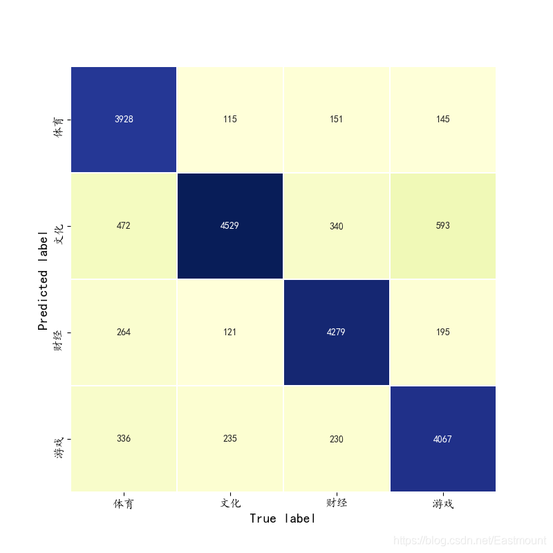
[[3928  472  264  336]
 [ 115 4529  121  235]
 [ 151  340 4279  230]
 [ 145  593  195 4067]]
             precision    recall  f1-score   support

          0       0.91      0.79      0.84      5000
          1       0.76      0.91      0.83      5000
          2       0.88      0.86      0.87      5000
          3       0.84      0.81      0.82      5000

avg / total       0.85      0.84      0.84     20000

             precision    recall  f1-score   support

          0       0.90      0.77      0.83      5000
          1       0.78      0.92      0.84      5000
          2       0.88      0.85      0.86      5000
          3       0.84      0.85      0.85      5000

avg / total       0.85      0.85      0.85     20000
IV TextCNN Chinese text classification
1. Principle introduction
TextCNN is an algorithm for text classification using convolutional neural network, which was proposed by Yoon Kim in the article "revolutionary neural networks for sense classification" in 2014.
The core idea of convolutional neural network is to capture local features. For text, local features are sliding windows composed of several words, similar to N-gram. The advantage of convolutional neural network is that it can automatically combine and screen N-gram features to obtain semantic information at different levels of abstraction. The following figure is the convolution neural network model architecture used for text classification in this paper.
Another classic paper of TextCNN is A Sensitivity Analysis of (and Practitioners' Guide to) revolutionary neural networks for sensitivity classification. The model results are shown in the figure below. TextCNN structure description, which is mainly used for text classification task, explains in detail how TextCNN architecture and word vector matrix convolute.
Suppose we have some sentences that need to be classified. Each word in the sentence is composed of an n-dimensional word vector, that is, the size of the input matrix is m*n, where m is the length of the sentence. CNN needs to convolute the input samples. For text data, the filter no longer slides horizontally, but only moves downward, which is somewhat similar to N-gram in extracting the local correlation between words.
There are three step strategies in the figure, namely 2, 3 and 4. Each step has two filters (there will be a large number of filters during actual training). Using different filters on different word windows, six convoluted vectors are finally obtained. Then, each vector is maximized and pooled, and each pooled value is spliced. Finally, the feature representation of the sentence is obtained. The sentence vector is thrown to the classifier for classification, and finally the whole text classification process is completed.
Finally, I sincerely recommend the following leaders' introduction to TextCNN, especially the Asia Lee boss of CSDN. I like his article very much. It's really great!
- <Convolutional Neural Networks for Sentence Classification2014>
- <A Sensitivity Analysis of (and Practitioners' Guide to) Convolutional Neural Networks for Sentence Classification>
- https://blog.csdn.net/asialee_bird/article/details/88813385
- https://zhuanlan.zhihu.com/p/77634533
2. Code implementation
The TextCNN code used by Keras to realize text classification is as follows:
- Keras_TextCNN_cnews.py
# -*- coding: utf-8 -*-
"""
Created on 2021-03-19
@author: xiuzhang Eastmount CSDN
TextCNN Model
"""
import os
import time
import pickle
import pandas as pd
import numpy as np
from sklearn import metrics
import matplotlib.pyplot as plt
import seaborn as sns
import tensorflow as tf
from sklearn.preprocessing import LabelEncoder,OneHotEncoder
from keras.models import Model
from keras.layers import LSTM, Activation, Dense, Dropout, Input, Embedding
from keras.layers import Convolution1D, MaxPool1D, Flatten
from keras.preprocessing.text import Tokenizer
from keras.preprocessing import sequence
from keras.callbacks import EarlyStopping
from keras.models import load_model
from keras.models import Sequential
from keras.layers.merge import concatenate

## If the GPU processing reader is a CPU, you can comment on this part of the code
## Specifies the maximum amount of video memory used in each GPU process 0.9 Indicates that it can be used GPU 90%Training with resources
os.environ["CUDA_DEVICES_ORDER"] = "PCI_BUS_IS"
os.environ["CUDA_VISIBLE_DEVICES"] = "0"
gpu_options = tf.GPUOptions(per_process_gpu_memory_fraction=0.8)
sess = tf.Session(config=tf.ConfigProto(gpu_options=gpu_options))

start = time.clock()

#----------------------------Step 1 data reading----------------------------
## Read test data set
train_df = pd.read_csv("news_dataset_train_fc.csv")
val_df = pd.read_csv("news_dataset_val_fc.csv")
test_df = pd.read_csv("news_dataset_test_fc.csv")

## Solve the problem of Chinese display
plt.rcParams['font.sans-serif'] = ['KaiTi']  #Specifies the default font SimHei bold
plt.rcParams['axes.unicode_minus'] = False   #Solution: the saved image is a negative sign'

#--------------------------Step 2 OneHotEncoder()code--------------------
## Encode the label data of the dataset
train_y = train_df.label
val_y = val_df.label
test_y = test_df.label
print("Label:")
print(train_y[:10])

le = LabelEncoder()
train_y = le.fit_transform(train_y).reshape(-1,1)
val_y = le.transform(val_y).reshape(-1,1)
test_y = le.transform(test_y).reshape(-1,1)
print("LabelEncoder")
print(train_y[:10])
print(len(train_y))

## Label data of the dataset-hot code
ohe = OneHotEncoder()
train_y = ohe.fit_transform(train_y).toarray()
val_y = ohe.transform(val_y).toarray()
test_y = ohe.transform(test_y).toarray()
print("OneHotEncoder:")
print(train_y[:10])

#-----------------------Step 3 use Tokenizer Encode phrases--------------------
max_words = 6000
max_len = 600
tok = Tokenizer(num_words=max_words)  #The maximum number of words is 6000
print(train_df.cutword[:5])
print(type(train_df.cutword))

## Prevent digital str processing in Corpus
train_content = [str(a) for a in train_df.cutword.tolist()]
val_content = [str(a) for a in val_df.cutword.tolist()]
test_content = [str(a) for a in test_df.cutword.tolist()]
tok.fit_on_texts(train_content)
print(tok)

## Save the trained Tokenizer and import
with open('tok.pickle', 'wb') as handle: #saving
    pickle.dump(tok, handle, protocol=pickle.HIGHEST_PROTOCOL)
with open('tok.pickle', 'rb') as handle: #loading
    tok = pickle.load(handle)

#---------------------------Step 4 convert data into sequence-----------------------------
train_seq = tok.texts_to_sequences(train_content)
val_seq = tok.texts_to_sequences(val_content)
test_seq = tok.texts_to_sequences(test_content)

## Adjust each sequence to the same length
train_seq_mat = sequence.pad_sequences(train_seq,maxlen=max_len)
val_seq_mat = sequence.pad_sequences(val_seq,maxlen=max_len)
test_seq_mat = sequence.pad_sequences(test_seq,maxlen=max_len)
print("Data conversion sequence")
print(train_seq_mat.shape)
print(val_seq_mat.shape)
print(test_seq_mat.shape)
print(train_seq_mat[:2])

#-------------------------------Step 5 establish TextCNN Model--------------------------
## 4 categories
num_labels = 4
inputs = Input(name='inputs',shape=[max_len], dtype='float64')
## Word embedding uses pre trained word vectors
layer = Embedding(max_words+1, 256, input_length=max_len, trainable=False)(inputs)
## The word window size is 3 respectively,4,5
cnn1 = Convolution1D(256, 3, padding='same', strides = 1, activation='relu')(layer)
cnn1 = MaxPool1D(pool_size=4)(cnn1)
cnn2 = Convolution1D(256, 4, padding='same', strides = 1, activation='relu')(layer)
cnn2 = MaxPool1D(pool_size=4)(cnn2)
cnn3 = Convolution1D(256, 5, padding='same', strides = 1, activation='relu')(layer)
cnn3 = MaxPool1D(pool_size=4)(cnn3)

# Merge the output vectors of the three models
cnn = concatenate([cnn1,cnn2,cnn3], axis=-1)
flat = Flatten()(cnn)
drop = Dropout(0.2)(flat)
main_output = Dense(num_labels, activation='softmax')(drop)
model = Model(inputs=inputs, outputs=main_output)
model.summary()
model.compile(loss="categorical_crossentropy",
              optimizer='adam',      # RMSprop()
              metrics=["accuracy"])

#-------------------------------Step 6 model training and prediction--------------------------
## First set to train training and then set to test test
flag = "train"
if flag == "train":
    print("model training")
    ## Model training-loss Stop training when you no longer improve 0.0001
    model_fit = model.fit(train_seq_mat, train_y, batch_size=128, epochs=10,
                          validation_data=(val_seq_mat,val_y),
                          callbacks=[EarlyStopping(monitor='val_loss',min_delta=0.0001)]
                         )
    model.save('my_model.h5')
    del model
    elapsed = (time.clock() - start)
    print("Time used:", elapsed)
    print(model_fit.history)

else:
    print("model prediction ")
    ## Import the trained model
    model = load_model('my_model.h5')
    ## Predict the test set
    test_pre = model.predict(test_seq_mat)
    ## Evaluate the prediction effect and calculate the confusion matrix
    confm = metrics.confusion_matrix(np.argmax(test_y,axis=1),np.argmax(test_pre,axis=1))
    print(confm)

    ## Confusion matrix visualization
    Labname = ["Sports", "Culture", "Finance and Economics", "game"]
    print(metrics.classification_report(np.argmax(test_y,axis=1),np.argmax(test_pre,axis=1)))
    plt.figure(figsize=(8,8))
    sns.heatmap(confm.T, square=True, annot=True,
                fmt='d', cbar=False, linewidths=.6,
                cmap="YlGnBu")
    plt.xlabel('True label',size = 14)
    plt.ylabel('Predicted label', size = 14)
    plt.xticks(np.arange(4)+0.5, Labname, size = 12)
    plt.yticks(np.arange(4)+0.5, Labname, size = 12)
    plt.savefig('result.png')
    plt.show()

    #----------------------------------Seventh, verify the algorithm--------------------------
    ## tok is used to preprocess the validation data set, and the trained model is used for prediction
    val_seq = tok.texts_to_sequences(val_df.cutword)
    ## Adjust each sequence to the same length
    val_seq_mat = sequence.pad_sequences(val_seq,maxlen=max_len)
    ## Predict validation set
    val_pre = model.predict(val_seq_mat)
    print(metrics.classification_report(np.argmax(val_y,axis=1),np.argmax(val_pre,axis=1)))
    elapsed = (time.clock() - start)
    print("Time used:", elapsed)
The training model is as follows:
__________________________________________________________________________________________________
Layer (type)                    Output Shape         Param #     Connected to
==================================================================================================
inputs (InputLayer)             (None, 600)          0
__________________________________________________________________________________________________
embedding_1 (Embedding)         (None, 600, 256)     1536256     inputs[0][0]
__________________________________________________________________________________________________
conv1d_1 (Conv1D)               (None, 600, 256)     196864      embedding_1[0][0]
__________________________________________________________________________________________________
conv1d_2 (Conv1D)               (None, 600, 256)     262400      embedding_1[0][0]
__________________________________________________________________________________________________
conv1d_3 (Conv1D)               (None, 600, 256)     327936      embedding_1[0][0]
__________________________________________________________________________________________________
max_pooling1d_1 (MaxPooling1D)  (None, 150, 256)     0           conv1d_1[0][0]
__________________________________________________________________________________________________
max_pooling1d_2 (MaxPooling1D)  (None, 150, 256)     0           conv1d_2[0][0]
__________________________________________________________________________________________________
max_pooling1d_3 (MaxPooling1D)  (None, 150, 256)     0           conv1d_3[0][0]
__________________________________________________________________________________________________
concatenate_1 (Concatenate)     (None, 150, 768)     0           max_pooling1d_1[0][0]
                                                                 max_pooling1d_2[0][0]
                                                                 max_pooling1d_3[0][0]
__________________________________________________________________________________________________
flatten_1 (Flatten)             (None, 115200)       0           concatenate_1[0][0]
__________________________________________________________________________________________________
dropout_1 (Dropout)             (None, 115200)       0           flatten_1[0][0]
__________________________________________________________________________________________________
dense_1 (Dense)                 (None, 4)            460804      dropout_1[0][0]
==================================================================================================
Total params: 2,784,260
Trainable params: 1,248,004
Non-trainable params: 1,536,256
__________________________________________________________________________________________________
The predicted results are as follows:
[[4448  238  182  132]
 [ 151 4572  124  153]
 [ 185  176 4545   94]
 [ 181  394  207 4218]]
             precision    recall  f1-score   support

          0       0.90      0.89      0.89      5000
          1       0.85      0.91      0.88      5000
          2       0.90      0.91      0.90      5000
          3       0.92      0.84      0.88      5000

avg / total       0.89      0.89      0.89     20000

             precision    recall  f1-score   support

          0       0.90      0.88      0.89      5000
          1       0.86      0.93      0.89      5000
          2       0.91      0.89      0.90      5000
          3       0.92      0.88      0.90      5000

avg / total       0.90      0.90      0.90     20000
V LSTM Chinese text classification
1. Principle introduction
Long Short Term network (LSTM) is a special type of RNN (Recurrent Neural Network), which can learn long-term dependence information. LSTM was proposed by Hochreiter & schmidhuber (1997) and recently improved and popularized by Alex Graves. In many problems, LSTM has achieved considerable success and has been widely used.
Because RNN has the problem of gradient disappearance, people have improved the hidden structure of sequence index position t. some techniques are used to make the hidden structure complex to avoid the problem of gradient disappearance. Such a special RNN is our LSTM. The full name of LSTM is long short term memory. Because of its design characteristics, LSTM is very suitable for modeling time series data, such as text data. The structure of LSTM is shown in the figure below:
LSTM is deliberately designed to avoid long-term dependency problems. Remember that long-term information is the default behavior of LSTM in practice, not the ability to obtain it at a great cost. LSTM has made some improvements on the ordinary RNN. LSTM RNN has three more controllers, namely:
- Input controller
- Output controller
- Forget controller
There are more mainlines on the left, such as the main plot of the film, while the original RNN system has become a branch plot, and the three controllers are on the branch.
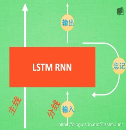
- Input controller (write gate): set a gate when inputting input. The function of gate is to judge whether to write this input into our Memory. It is equivalent to a parameter and can be trained. This parameter is used to control whether to remember the current point.
- Output controller (read gate): in the gate of the output position, judge whether to read the current Memory.
- Forget gate: the forget gate of the processing position to determine whether to forget the previous Memory.
The working principle of LSTM is: if the branch content is very important for the final result, the input controller will write the branch content into the main line content according to the importance, and then analyze it; If the branching content changes our previous idea, the forgetting controller will forget some mainline content and replace the new content proportionally, so the update of mainline content depends on input and forgetting control; The final output will be based on the main line content and branch line content. Through these three gate s, we can well control our RNN. Based on these control mechanisms, LSTM is a good medicine to delay memory, so as to bring better results.
2. Code implementation
The LSTM code of text classification implemented by Keras is as follows:
- Keras_LSTM_cnews.py
"""
Created on 2021-03-19
@author: xiuzhang Eastmount CSDN
LSTM Model
"""
import os
import time
import pickle
import pandas as pd
import numpy as np
from sklearn import metrics
import matplotlib.pyplot as plt
import seaborn as sns
import tensorflow as tf
from sklearn.preprocessing import LabelEncoder,OneHotEncoder
from keras.models import Model
from keras.layers import LSTM, Activation, Dense, Dropout, Input, Embedding
from keras.layers import Convolution1D, MaxPool1D, Flatten
from keras.preprocessing.text import Tokenizer
from keras.preprocessing import sequence
from keras.callbacks import EarlyStopping
from keras.models import load_model
from keras.models import Sequential

#GPU accelerates CuDNNLSTM faster than LSTM
from keras.layers import CuDNNLSTM, CuDNNGRU

## If the GPU processing reader is a CPU, you can comment on this part of the code
## Specifies the maximum amount of video memory used in each GPU process 0.9 Indicates that it can be used GPU 90%Training with resources
os.environ["CUDA_DEVICES_ORDER"] = "PCI_BUS_IS"
os.environ["CUDA_VISIBLE_DEVICES"] = "0"
gpu_options = tf.GPUOptions(per_process_gpu_memory_fraction=0.8)
sess = tf.Session(config=tf.ConfigProto(gpu_options=gpu_options))

start = time.clock()

#----------------------------Step 1 data reading----------------------------
## Read test data set
train_df = pd.read_csv("news_dataset_train_fc.csv")
val_df = pd.read_csv("news_dataset_val_fc.csv")
test_df = pd.read_csv("news_dataset_test_fc.csv")
print(train_df.head())

## Solve the problem of Chinese display
plt.rcParams['font.sans-serif'] = ['KaiTi']  #Specifies the default font SimHei bold
plt.rcParams['axes.unicode_minus'] = False   #Solution: the saved image is a negative sign'

#--------------------------Step 2 OneHotEncoder()code--------------------
## Encode the label data of the dataset
train_y = train_df.label
val_y = val_df.label
test_y = test_df.label
print("Label:")
print(train_y[:10])

le = LabelEncoder()
train_y = le.fit_transform(train_y).reshape(-1,1)
val_y = le.transform(val_y).reshape(-1,1)
test_y = le.transform(test_y).reshape(-1,1)
print("LabelEncoder")
print(train_y[:10])
print(len(train_y))

## Label data of the dataset-hot code
ohe = OneHotEncoder()
train_y = ohe.fit_transform(train_y).toarray()
val_y = ohe.transform(val_y).toarray()
test_y = ohe.transform(test_y).toarray()
print("OneHotEncoder:")
print(train_y[:10])

#-----------------------Step 3 use Tokenizer Encode phrases--------------------
max_words = 6000
max_len = 600
tok = Tokenizer(num_words=max_words)  #The maximum number of words is 6000
print(train_df.cutword[:5])
print(type(train_df.cutword))

## Prevent digital str processing in Corpus
train_content = [str(a) for a in train_df.cutword.tolist()]
val_content = [str(a) for a in val_df.cutword.tolist()]
test_content = [str(a) for a in test_df.cutword.tolist()]
tok.fit_on_texts(train_content)
print(tok)

## Save the trained Tokenizer and import
with open('tok.pickle', 'wb') as handle: #saving
    pickle.dump(tok, handle, protocol=pickle.HIGHEST_PROTOCOL)
with open('tok.pickle', 'rb') as handle: #loading
    tok = pickle.load(handle)

#---------------------------Step 4 convert data into sequence-----------------------------
train_seq = tok.texts_to_sequences(train_content)
val_seq = tok.texts_to_sequences(val_content)
test_seq = tok.texts_to_sequences(test_content)

## Adjust each sequence to the same length
train_seq_mat = sequence.pad_sequences(train_seq,maxlen=max_len)
val_seq_mat = sequence.pad_sequences(val_seq,maxlen=max_len)
test_seq_mat = sequence.pad_sequences(test_seq,maxlen=max_len)
print("Data conversion sequence")
print(train_seq_mat.shape)
print(val_seq_mat.shape)
print(test_seq_mat.shape)
print(train_seq_mat[:2])

#-------------------------------Step 5 establish LSTM Model--------------------------
## Define LSTM model
inputs = Input(name='inputs',shape=[max_len],dtype='float64')
## Embedding (vocabulary size, batch size, word length of each news)
layer = Embedding(max_words+1, 128, input_length=max_len)(inputs)
#layer = LSTM(128)(layer)
layer = CuDNNLSTM(128)(layer)

layer = Dense(128, activation="relu", name="FC1")(layer)
layer = Dropout(0.1)(layer)
layer = Dense(4, activation="softmax", name="FC2")(layer)
model = Model(inputs=inputs, outputs=layer)
model.summary()
model.compile(loss="categorical_crossentropy",
              optimizer='adam',  # RMSprop()
              metrics=["accuracy"])

#-------------------------------Step 6 model training and prediction--------------------------
## First set to train training and then set to test test
flag = "train"
if flag == "train":
    print("model training")
    ## Model training-loss Stop training when you no longer improve 0.0001
    model_fit = model.fit(train_seq_mat, train_y, batch_size=128, epochs=10,
                          validation_data=(val_seq_mat,val_y),
                          callbacks=[EarlyStopping(monitor='val_loss',min_delta=0.0001)]
                         )
    model.save('my_model.h5')
    del model
    elapsed = (time.clock() - start)
    print("Time used:", elapsed)
    print(model_fit.history)

else:
    print("model prediction ")
    ## Import the trained model
    model = load_model('my_model.h5')
    ## Predict the test set
    test_pre = model.predict(test_seq_mat)
    ## Evaluate the prediction effect and calculate the confusion matrix
    confm = metrics.confusion_matrix(np.argmax(test_y,axis=1),np.argmax(test_pre,axis=1))
    print(confm)

    ## Confusion matrix visualization
    Labname = ["Sports", "Culture", "Finance and Economics", "game"]
    print(metrics.classification_report(np.argmax(test_y,axis=1),np.argmax(test_pre,axis=1)))
    plt.figure(figsize=(8,8))
    sns.heatmap(confm.T, square=True, annot=True,
                fmt='d', cbar=False, linewidths=.6,
                cmap="YlGnBu")
    plt.xlabel('True label',size = 14)
    plt.ylabel('Predicted label', size = 14)
    plt.xticks(np.arange(4)+0.8, Labname, size = 12)
    plt.yticks(np.arange(4)+0.4, Labname, size = 12)
    plt.savefig('result.png')
    plt.show()

    #----------------------------------Seventh, verify the algorithm--------------------------
    ## tok is used to preprocess the validation data set, and the trained model is used for prediction
    val_seq = tok.texts_to_sequences(val_df.cutword)
    ## Adjust each sequence to the same length
    val_seq_mat = sequence.pad_sequences(val_seq,maxlen=max_len)
    ## Predict validation set
    val_pre = model.predict(val_seq_mat)
    print(metrics.classification_report(np.argmax(val_y,axis=1),np.argmax(val_pre,axis=1)))
    elapsed = (time.clock() - start)
    print("Time used:", elapsed)
The training output model is as follows:
_________________________________________________________________
Layer (type)                 Output Shape              Param #
=================================================================
inputs (InputLayer)          (None, 600)               0
_________________________________________________________________
embedding_1 (Embedding)      (None, 600, 128)          768128
_________________________________________________________________
cu_dnnlstm_1 (CuDNNLSTM)     (None, 128)               132096
_________________________________________________________________
FC1 (Dense)                  (None, 128)               16512
_________________________________________________________________
dropout_1 (Dropout)          (None, 128)               0
_________________________________________________________________
FC2 (Dense)                  (None, 4)                 516
=================================================================
Total params: 917,252
Trainable params: 917,252
Non-trainable params: 0
The predicted results are as follows:
[[4539  153  188  120]
 [  47 4628  181  144]
 [ 113  133 4697   57]
 [ 101  292  157 4450]]
             precision    recall  f1-score   support

          0       0.95      0.91      0.93      5000
          1       0.89      0.93      0.91      5000
          2       0.90      0.94      0.92      5000
          3       0.93      0.89      0.91      5000

avg / total       0.92      0.92      0.92     20000

             precision    recall  f1-score   support

          0       0.96      0.89      0.92      5000
          1       0.89      0.94      0.92      5000
          2       0.90      0.93      0.92      5000
          3       0.94      0.92      0.93      5000

avg / total       0.92      0.92      0.92     20000
Vi BiLSTM Chinese text classification
1. Principle introduction
BiLSTM is the abbreviation of bi directional long short term memory, which is a combination of forward LSTM and backward LSTM. Both it and LSTM are often used to model context information in natural language processing tasks. The forward LSTM is combined with the backward LSTM to form the BiLSTM. For example, we code the sentence "I love China", and the model is shown in the figure.
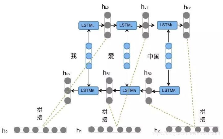
There is still a problem in using LSTM to model sentences: it is impossible to encode back to front information. In more fine-grained classification, such as the five classification tasks of strong commendatory meaning, weak commendatory meaning, neutral, weak derogatory meaning and strong derogatory meaning, we need to pay attention to the interaction between emotional words, degree words and negative words. For example, "this restaurant is not as dirty as the next door". The "no" here is a modification of the degree of "dirty". BiLSTM can better capture the two-way semantic dependence.
- Reference article: https://zhuanlan.zhihu.com/p/47802053
2. Code implementation
The BiLSTM code that Keras implements text classification is as follows:
- Keras_BiLSTM_cnews.py
"""
Created on 2021-03-19
@author: xiuzhang Eastmount CSDN
BiLSTM Model
"""
import os
import time
import pickle
import pandas as pd
import numpy as np
from sklearn import metrics
import matplotlib.pyplot as plt
import seaborn as sns
import tensorflow as tf
from sklearn.preprocessing import LabelEncoder,OneHotEncoder
from keras.models import Model
from keras.layers import LSTM, Activation, Dense, Dropout, Input, Embedding
from keras.layers import Convolution1D, MaxPool1D, Flatten
from keras.preprocessing.text import Tokenizer
from keras.preprocessing import sequence
from keras.callbacks import EarlyStopping
from keras.models import load_model
from keras.models import Sequential

#GPU accelerates CuDNNLSTM faster than LSTM
from keras.layers import CuDNNLSTM, CuDNNGRU
from keras.layers import Bidirectional

## If the GPU processing reader is a CPU, you can comment on this part of the code
## Specifies the maximum amount of video memory used in each GPU process 0.9 Indicates that it can be used GPU 90%Training with resources
os.environ["CUDA_DEVICES_ORDER"] = "PCI_BUS_IS"
os.environ["CUDA_VISIBLE_DEVICES"] = "0"
gpu_options = tf.GPUOptions(per_process_gpu_memory_fraction=0.8)
sess = tf.Session(config=tf.ConfigProto(gpu_options=gpu_options))

start = time.clock()

#----------------------------Step 1 data reading----------------------------
## Read test data set
train_df = pd.read_csv("news_dataset_train_fc.csv")
val_df = pd.read_csv("news_dataset_val_fc.csv")
test_df = pd.read_csv("news_dataset_test_fc.csv")
print(train_df.head())

## Solve the problem of Chinese display
plt.rcParams['font.sans-serif'] = ['KaiTi']  #Specifies the default font SimHei bold
plt.rcParams['axes.unicode_minus'] = False   #Solution: the saved image is a negative sign'

#--------------------------Step 2 OneHotEncoder()code--------------------
## Encode the label data of the dataset
train_y = train_df.label
val_y = val_df.label
test_y = test_df.label
print("Label:")
print(train_y[:10])

le = LabelEncoder()
train_y = le.fit_transform(train_y).reshape(-1,1)
val_y = le.transform(val_y).reshape(-1,1)
test_y = le.transform(test_y).reshape(-1,1)
print("LabelEncoder")
print(train_y[:10])
print(len(train_y))

## Label data of the dataset-hot code
ohe = OneHotEncoder()
train_y = ohe.fit_transform(train_y).toarray()
val_y = ohe.transform(val_y).toarray()
test_y = ohe.transform(test_y).toarray()
print("OneHotEncoder:")
print(train_y[:10])

#-----------------------Step 3 use Tokenizer Encode phrases--------------------
max_words = 6000
max_len = 600
tok = Tokenizer(num_words=max_words)  #The maximum number of words is 6000
print(train_df.cutword[:5])
print(type(train_df.cutword))

## Prevent digital str processing in Corpus
train_content = [str(a) for a in train_df.cutword.tolist()]
val_content = [str(a) for a in val_df.cutword.tolist()]
test_content = [str(a) for a in test_df.cutword.tolist()]
tok.fit_on_texts(train_content)
print(tok)

## Save the trained Tokenizer and import
with open('tok.pickle', 'wb') as handle: #saving
    pickle.dump(tok, handle, protocol=pickle.HIGHEST_PROTOCOL)
with open('tok.pickle', 'rb') as handle: #loading
    tok = pickle.load(handle)

#---------------------------Step 4 convert data into sequence-----------------------------
train_seq = tok.texts_to_sequences(train_content)
val_seq = tok.texts_to_sequences(val_content)
test_seq = tok.texts_to_sequences(test_content)

## Adjust each sequence to the same length
train_seq_mat = sequence.pad_sequences(train_seq,maxlen=max_len)
val_seq_mat = sequence.pad_sequences(val_seq,maxlen=max_len)
test_seq_mat = sequence.pad_sequences(test_seq,maxlen=max_len)
print("Data conversion sequence")
print(train_seq_mat.shape)
print(val_seq_mat.shape)
print(test_seq_mat.shape)
print(train_seq_mat[:2])

#-------------------------------Step 5 establish BiLSTM Model--------------------------
num_labels = 4
model = Sequential()
model.add(Embedding(max_words+1, 128, input_length=max_len))
model.add(Bidirectional(CuDNNLSTM(128)))
model.add(Dense(128, activation='relu'))
model.add(Dropout(0.3))
model.add(Dense(num_labels, activation='softmax'))
model.summary()
model.compile(loss="categorical_crossentropy",
              optimizer='adam',  # RMSprop()
              metrics=["accuracy"])

#-------------------------------Step 6 model training and prediction--------------------------
## First set to train training and then set to test test
flag = "train"
if flag == "train":
    print("model training")
    ## Model training-loss Stop training when you no longer improve 0.0001
    model_fit = model.fit(train_seq_mat, train_y, batch_size=128, epochs=10,
                          validation_data=(val_seq_mat,val_y),
                          callbacks=[EarlyStopping(monitor='val_loss',min_delta=0.0001)]
                         )
    model.save('my_model.h5')
    del model
    elapsed = (time.clock() - start)
    print("Time used:", elapsed)
    print(model_fit.history)

else:
    print("model prediction ")
    ## Import the trained model
    model = load_model('my_model.h5')
    ## Predict the test set
    test_pre = model.predict(test_seq_mat)
    ## Evaluate the prediction effect and calculate the confusion matrix
    confm = metrics.confusion_matrix(np.argmax(test_y,axis=1),np.argmax(test_pre,axis=1))
    print(confm)

    ## Confusion matrix visualization
    Labname = ["Sports", "Culture", "Finance and Economics", "game"]
    print(metrics.classification_report(np.argmax(test_y,axis=1),np.argmax(test_pre,axis=1)))
    plt.figure(figsize=(8,8))
    sns.heatmap(confm.T, square=True, annot=True,
                fmt='d', cbar=False, linewidths=.6,
                cmap="YlGnBu")
    plt.xlabel('True label',size = 14)
    plt.ylabel('Predicted label', size = 14)
    plt.xticks(np.arange(4)+0.5, Labname, size = 12)
    plt.yticks(np.arange(4)+0.5, Labname, size = 12)
    plt.savefig('result.png')
    plt.show()

    #----------------------------------Seventh, verify the algorithm--------------------------
    ## tok is used to preprocess the validation data set, and the trained model is used for prediction
    val_seq = tok.texts_to_sequences(val_df.cutword)
    ## Adjust each sequence to the same length
    val_seq_mat = sequence.pad_sequences(val_seq,maxlen=max_len)
    ## Predict validation set
    val_pre = model.predict(val_seq_mat)
    print(metrics.classification_report(np.argmax(val_y,axis=1),np.argmax(val_pre,axis=1)))
    elapsed = (time.clock() - start)
    print("Time used:", elapsed)
The training output model is shown below, and the GPU time is still very fast.
_________________________________________________________________
Layer (type)                 Output Shape              Param #
=================================================================
embedding_1 (Embedding)      (None, 600, 128)          768128
_________________________________________________________________
bidirectional_1 (Bidirection (None, 256)               264192
_________________________________________________________________
dense_1 (Dense)              (None, 128)               32896
_________________________________________________________________
dropout_1 (Dropout)          (None, 128)               0
_________________________________________________________________
dense_2 (Dense)              (None, 4)                 516
=================================================================
Total params: 1,065,732
Trainable params: 1,065,732
Non-trainable params: 0

Train on 40000 samples, validate on 20000 samples
Epoch 1/10
40000/40000 [==============================] - 23s 587us/step - loss: 0.5825 - acc: 0.8038 - val_loss: 0.2321 - val_acc: 0.9246
Epoch 2/10
40000/40000 [==============================] - 21s 521us/step - loss: 0.1433 - acc: 0.9542 - val_loss: 0.2422 - val_acc: 0.9228
Time used: 52.763230400000005
The prediction results are shown in the figure below:

[[4593  143  113  151]
 [  81 4679   60  180]
 [ 110  199 4590  101]
 [  73  254   82 4591]]
             precision    recall  f1-score   support

          0       0.95      0.92      0.93      5000
          1       0.89      0.94      0.91      5000
          2       0.95      0.92      0.93      5000
          3       0.91      0.92      0.92      5000

avg / total       0.92      0.92      0.92     20000

             precision    recall  f1-score   support

          0       0.94      0.90      0.92      5000
          1       0.89      0.95      0.92      5000
          2       0.95      0.90      0.93      5000
          3       0.91      0.94      0.93      5000

avg / total       0.92      0.92      0.92     20000
VII BiLSTM+Attention Chinese text classification
1. Principle introduction
Attention mechanism is a problem-solving method proposed by imitating human attention. In short, it is to quickly screen out high-value information from a large amount of information. It is mainly used to solve the problem that it is difficult to obtain the final reasonable vector representation when the input sequence of LSTM/RNN model is long. The method is to retain the intermediate result of LSTM, learn it with a new model, and associate it with the output, so as to achieve the purpose of information screening.
What is attention?
First, briefly describe what the attention mechanism is. I believe NLP students will not be unfamiliar with this mechanism. It can be said to shine in the paper "Attention is all you need". In the machine translation task, it helped the depth model greatly improve its performance and output the best state of art model at that time. Of course, in addition to the attention mechanism, the model also uses many useful trick s to help improve the performance of the model. However, it cannot be denied that the core of this model is attention.
Attention mechanism, also known as attention mechanism, is a technology that enables the model to focus on important information and fully learn and absorb. It is not a complete model, but a technology that can act on any sequence model.
Why attention?
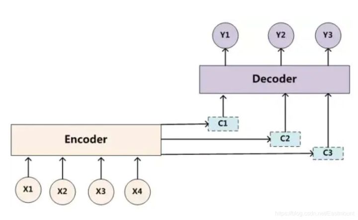
Why introduce the attention mechanism. For example, in the seq2seq model, for a text sequence, we usually use some mechanism to encode the sequence, encode it into a fixed length vector through dimension reduction and other methods, and input it to the subsequent full connection layer. Generally, we will use CNN or RNN (including GRU or LSTM) and other models to encode the sequence data, and then use various pooling or RNN to directly take the hidden state at the last t time as the vector output of the sentence.
However, there will be a problem here: conventional coding methods can not reflect the attention to different morphemes in a sentence sequence. In natural language, different parts of a sentence have different meanings and importance. For example, in the above example: I hate this movie If you do emotional analysis, it is obvious that you should pay more attention to the word hate. Of course, CNN and RNN can encode this information, but there is also an upper limit on this coding ability. For longer texts, the model effect will not be improved too much.
- Reference and recommended articles: https://zhuanlan.zhihu.com/p/46313756
Attention has a wide range of applications, including text and pictures.
- Text: applied to the seq2seq model. The most common application is translation
- Image: image extraction applied to convolutional neural network
- voice
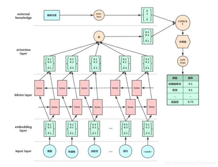
The following figure is a classic BiLSTM+Attention model, which is also the model we need to establish next.
2. Code implementation
The BiLSTM+Attention code used by Keras to realize text classification is as follows:
- Keras_Attention_BiLSTM_cnews.py
"""
Created on 2021-03-19
@author: xiuzhang Eastmount CSDN
BiLSTM+Attention Model
"""
import os
import time
import pickle
import pandas as pd
import numpy as np
from sklearn import metrics
import matplotlib.pyplot as plt
import seaborn as sns
import tensorflow as tf
from sklearn.preprocessing import LabelEncoder,OneHotEncoder
from keras.models import Model
from keras.layers import LSTM, Activation, Dense, Dropout, Input, Embedding
from keras.layers import Convolution1D, MaxPool1D, Flatten
from keras.preprocessing.text import Tokenizer
from keras.preprocessing import sequence
from keras.callbacks import EarlyStopping
from keras.models import load_model
from keras.models import Sequential

#GPU accelerates CuDNNLSTM faster than LSTM
from keras.layers import CuDNNLSTM, CuDNNGRU
from keras.layers import Bidirectional

## If the GPU processing reader is a CPU, you can comment on this part of the code
## Specifies the maximum amount of video memory used in each GPU process 0.9 Indicates that it can be used GPU 90%Training with resources
os.environ["CUDA_DEVICES_ORDER"] = "PCI_BUS_IS"
os.environ["CUDA_VISIBLE_DEVICES"] = "0"
gpu_options = tf.GPUOptions(per_process_gpu_memory_fraction=0.8)
sess = tf.Session(config=tf.ConfigProto(gpu_options=gpu_options))

start = time.clock()

#----------------------------Step 1 data reading----------------------------
## Read test data set
train_df = pd.read_csv("news_dataset_train_fc.csv")
val_df = pd.read_csv("news_dataset_val_fc.csv")
test_df = pd.read_csv("news_dataset_test_fc.csv")
print(train_df.head())

## Solve the problem of Chinese display
plt.rcParams['font.sans-serif'] = ['KaiTi']  #Specifies the default font SimHei bold
plt.rcParams['axes.unicode_minus'] = False   #Solution: the saved image is a negative sign'

#--------------------------Step 2 OneHotEncoder()code--------------------
## Encode the label data of the dataset
train_y = train_df.label
val_y = val_df.label
test_y = test_df.label
print("Label:")
print(train_y[:10])

le = LabelEncoder()
train_y = le.fit_transform(train_y).reshape(-1,1)
val_y = le.transform(val_y).reshape(-1,1)
test_y = le.transform(test_y).reshape(-1,1)
print("LabelEncoder")
print(train_y[:10])
print(len(train_y))

## Label data of the dataset-hot code
ohe = OneHotEncoder()
train_y = ohe.fit_transform(train_y).toarray()
val_y = ohe.transform(val_y).toarray()
test_y = ohe.transform(test_y).toarray()
print("OneHotEncoder:")
print(train_y[:10])

#-----------------------Step 3 use Tokenizer Encode phrases--------------------
max_words = 6000
max_len = 600
tok = Tokenizer(num_words=max_words)  #The maximum number of words is 6000
print(train_df.cutword[:5])
print(type(train_df.cutword))

## Prevent digital str processing in Corpus
train_content = [str(a) for a in train_df.cutword.tolist()]
val_content = [str(a) for a in val_df.cutword.tolist()]
test_content = [str(a) for a in test_df.cutword.tolist()]
tok.fit_on_texts(train_content)
print(tok)

## Save the trained Tokenizer and import
with open('tok.pickle', 'wb') as handle: #saving
    pickle.dump(tok, handle, protocol=pickle.HIGHEST_PROTOCOL)
with open('tok.pickle', 'rb') as handle: #loading
    tok = pickle.load(handle)

#---------------------------Step 4 convert data into sequence-----------------------------
train_seq = tok.texts_to_sequences(train_content)
val_seq = tok.texts_to_sequences(val_content)
test_seq = tok.texts_to_sequences(test_content)

## Adjust each sequence to the same length
train_seq_mat = sequence.pad_sequences(train_seq,maxlen=max_len)
val_seq_mat = sequence.pad_sequences(val_seq,maxlen=max_len)
test_seq_mat = sequence.pad_sequences(test_seq,maxlen=max_len)
print("Data conversion sequence")
print(train_seq_mat.shape)
print(val_seq_mat.shape)
print(test_seq_mat.shape)
print(train_seq_mat[:2])

#---------------------------Step 5 establish Attention mechanism----------------------
"""
because Keras There is no ready-made Attention Layer can be used directly. We need to build a new layer function ourselves.
Keras The user-defined function is mainly divided into four parts:
init: Initialize some required parameters
bulid: How to define the weight
call: The core part defines how vectors operate
compute_output_shape: Defines the size of the layer's output
 Recommended articles:
    https://blog.csdn.net/huanghaocs/article/details/95752379
    https://zhuanlan.zhihu.com/p/29201491
"""

# Hierarchical Model with Attention
from keras import initializers
from keras import constraints
from keras import activations
from keras import regularizers
from keras import backend as K
from keras.engine.topology import Layer

K.clear_session()

class AttentionLayer(Layer):
    def __init__(self, attention_size=None, **kwargs):
        self.attention_size = attention_size
        super(AttentionLayer, self).__init__(**kwargs)

    def get_config(self):
        config = super().get_config()
        config['attention_size'] = self.attention_size
        return config

    def build(self, input_shape):
        assert len(input_shape) == 3

        self.time_steps = input_shape[1]
        hidden_size = input_shape[2]
        if self.attention_size is None:
            self.attention_size = hidden_size

        self.W = self.add_weight(name='att_weight', shape=(hidden_size, self.attention_size),
                                initializer='uniform', trainable=True)
        self.b = self.add_weight(name='att_bias', shape=(self.attention_size,),
                                initializer='uniform', trainable=True)
        self.V = self.add_weight(name='att_var', shape=(self.attention_size,),
                                initializer='uniform', trainable=True)
        super(AttentionLayer, self).build(input_shape)

    def call(self, inputs):
        self.V = K.reshape(self.V, (-1, 1))
        H = K.tanh(K.dot(inputs, self.W) + self.b)
        score = K.softmax(K.dot(H, self.V), axis=1)
        outputs = K.sum(score * inputs, axis=1)
        return outputs

    def compute_output_shape(self, input_shape):
        return input_shape[0], input_shape[2]

#-------------------------------Step 6 establish BiLSTM Model--------------------------
## Defining the BiLSTM model
## BiLSTM+Attention
num_labels = 4
inputs = Input(name='inputs',shape=[max_len],dtype='float64')
layer = Embedding(max_words+1, 256, input_length=max_len)(inputs)
#lstm = Bidirectional(LSTM(100, dropout=0.2, recurrent_dropout=0.1, return_sequences=True))(layer)
bilstm = Bidirectional(CuDNNLSTM(128, return_sequences=True))(layer)  #Parameter hold dimension 3
layer = Dense(128, activation='relu')(bilstm)
layer = Dropout(0.2)(layer)
## Attention mechanism
attention = AttentionLayer(attention_size=50)(layer)
output = Dense(num_labels, activation='softmax')(attention)
model = Model(inputs=inputs, outputs=output)
model.summary()
model.compile(loss="categorical_crossentropy",
              optimizer='adam',      # RMSprop()
              metrics=["accuracy"])

#-------------------------------Step 7 model training and prediction--------------------------
## First set to train training and then set to test test
flag = "test"
if flag == "train":
    print("model training")
    ## Model training-loss Stop training when you no longer improve 0.0001
    model_fit = model.fit(train_seq_mat, train_y, batch_size=128, epochs=10,
                          validation_data=(val_seq_mat,val_y),
                          callbacks=[EarlyStopping(monitor='val_loss',min_delta=0.0001)]
                         )
    ## Save model
    model.save('my_model.h5')
    del model  # deletes the existing model
    ## computing time
    elapsed = (time.clock() - start)
    print("Time used:", elapsed)
    print(model_fit.history)

else:
    print("model prediction ")
    ## Import the trained model
    model = load_model('my_model.h5', custom_objects={'AttentionLayer': AttentionLayer(50)}, compile=False)
    ## Predict the test set
    test_pre = model.predict(test_seq_mat)
    ## Evaluate the prediction effect and calculate the confusion matrix
    confm = metrics.confusion_matrix(np.argmax(test_y,axis=1),np.argmax(test_pre,axis=1))
    print(confm)

    ## Confusion matrix visualization
    Labname = ["Sports", "Culture", "Finance and Economics", "game"]
    print(metrics.classification_report(np.argmax(test_y,axis=1),np.argmax(test_pre,axis=1)))
    plt.figure(figsize=(8,8))
    sns.heatmap(confm.T, square=True, annot=True,
                fmt='d', cbar=False, linewidths=.6,
                cmap="YlGnBu")
    plt.xlabel('True label',size = 14)
    plt.ylabel('Predicted label', size = 14)
    plt.xticks(np.arange(4)+0.5, Labname, size = 12)
    plt.yticks(np.arange(4)+0.5, Labname, size = 12)
    plt.savefig('result.png')
    plt.show()

    #----------------------------------Seventh, verify the algorithm--------------------------
    ## tok is used to preprocess the validation data set, and the trained model is used for prediction
    val_seq = tok.texts_to_sequences(val_df.cutword)
    ## Adjust each sequence to the same length
    val_seq_mat = sequence.pad_sequences(val_seq,maxlen=max_len)
    ## Predict validation set
    val_pre = model.predict(val_seq_mat)
    print(metrics.classification_report(np.argmax(val_y,axis=1),np.argmax(val_pre,axis=1)))

    ## computing time
    elapsed = (time.clock() - start)
    print("Time used:", elapsed)
The training output model is as follows:
_________________________________________________________________
Layer (type)                 Output Shape              Param #
=================================================================
inputs (InputLayer)          (None, 600)               0
_________________________________________________________________
embedding_1 (Embedding)      (None, 600, 256)          1536256
_________________________________________________________________
bidirectional_1 (Bidirection (None, 600, 256)          395264
_________________________________________________________________
dense_1 (Dense)              (None, 600, 128)          32896
_________________________________________________________________
dropout_1 (Dropout)          (None, 600, 128)          0
_________________________________________________________________
attention_layer_1 (Attention (None, 128)               6500
_________________________________________________________________
dense_2 (Dense)              (None, 4)                 516
=================================================================
Total params: 1,971,432
Trainable params: 1,971,432
Non-trainable params: 0
The prediction results are shown in the figure below:
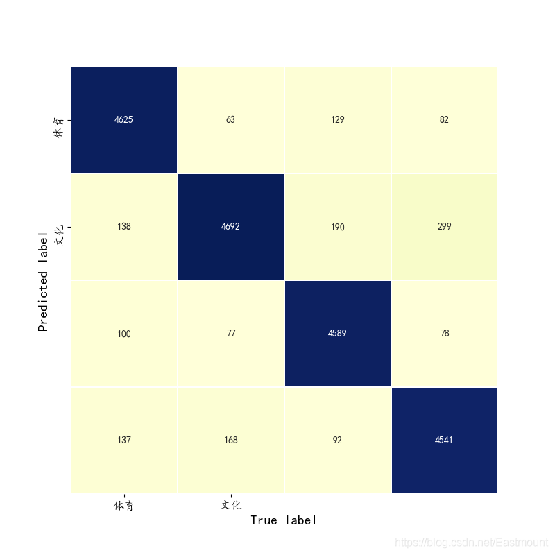
[[4625  138  100  137]
 [  63 4692   77  168]
 [ 129  190 4589   92]
 [  82  299   78 4541]]
             precision    recall  f1-score   support

          0       0.94      0.93      0.93      5000
          1       0.88      0.94      0.91      5000
          2       0.95      0.92      0.93      5000
          3       0.92      0.91      0.91      5000

avg / total       0.92      0.92      0.92     20000

             precision    recall  f1-score   support

          0       0.95      0.91      0.93      5000
          1       0.88      0.95      0.91      5000
          2       0.95      0.90      0.92      5000
          3       0.92      0.93      0.93      5000

avg / total       0.92      0.92      0.92     20000
Click focus to learn about Huawei cloud's new technologies for the first time~