Old readers should know that I have been speculating in stocks for more than two years.

From the initial fund to later stocks, the amount has been small, up to 300000.

At the best time of the rise, there is a floating profit of nearly 10000 every day, and occasionally there is a floating profit of nearly 20000.

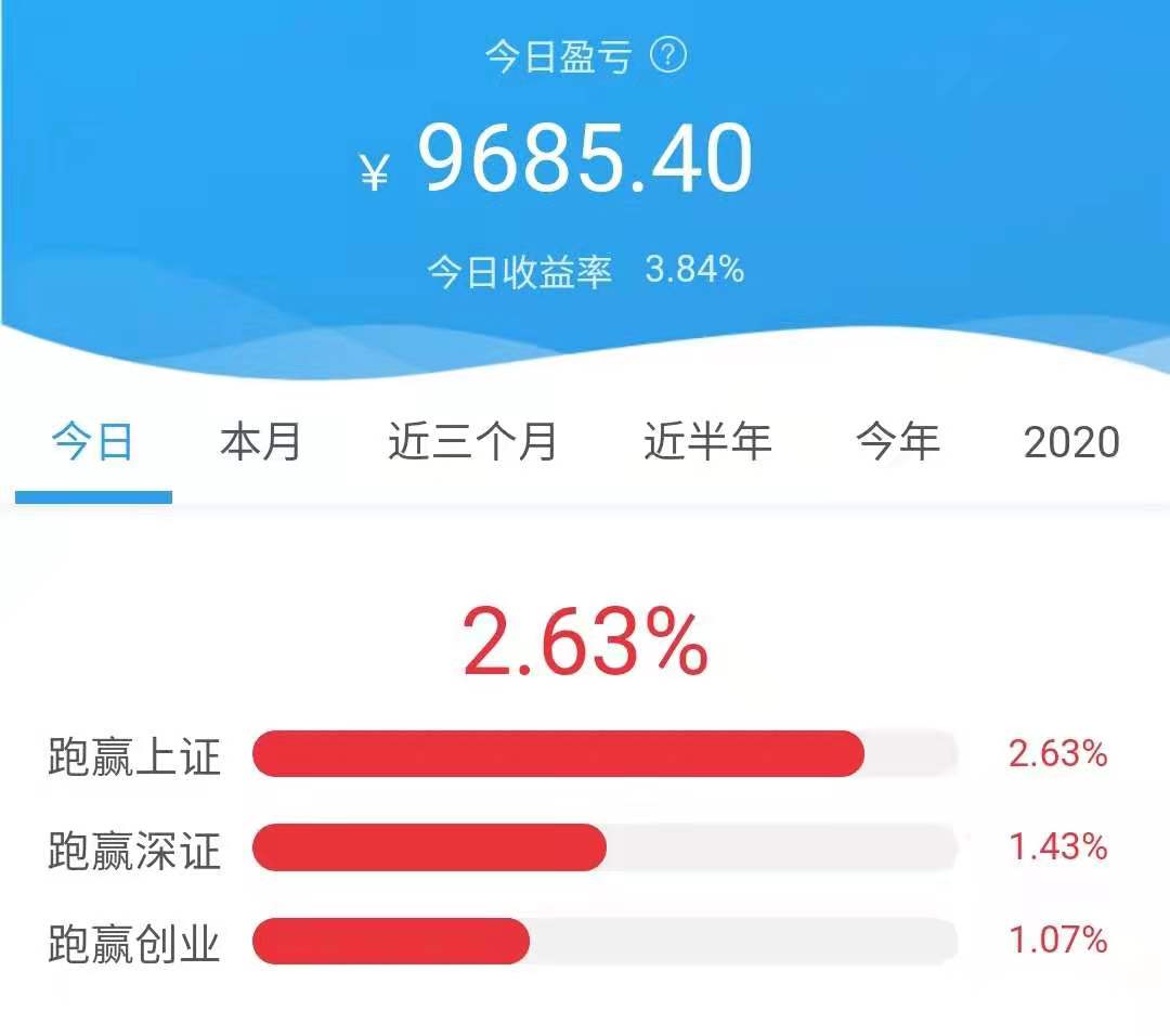
Since February this year, the stock market opened a difficult mode, such a good day has come to an end.

At the beginning of the year, tens of thousands of floating profits also lost more than half. In addition, this year, it is planned to use a lot of money and the body is hollowed out.

Stock market investment is a lot conservative, basically fixed at a low position of about 100000, focusing on participation.

There have always been readers who want to read my financial articles. At first, they promised, and then they thought about it carefully.

You said, I'm a technology blogger and write about financial management. Isn't that a dereliction of business?

Besides, I didn't study finance. Although I made some small money in the stock market by luck, after all, I'm not professional and don't dare to command disorderly.

Recently, I suddenly thought, financial management + technology, I can~

I like learning new knowledge very much. It is not limited to computer technology. I always keep a curiosity and want to learn everything.

As it happens, I plan to publish a video on quantitative trading in the near future to explore the application of artificial intelligence technology in investing in the stock market.

Learning, I found that the water in it was very deep, "I can't grasp it".

Quantitative trading is not as easy as I thought. There is a lot to learn.

One weekend, I entered the door.

Today, let's share the basic knowledge of quantitative trading and warm up the video.

Quantitative transaction

Quantitative trading is a securities investment method that uses computer technology to trade with the help of modern statistical and mathematical methods.

The main knowledge points covered are as follows:

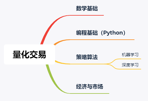
Mathematics, programming, finance and algorithms must be understood. It's OK where you can't make up.

Quantitative platform

Grasping data, writing strategies and online trading, if you do it alone, the cost is too high, which is not conducive to the initial learning.

I have investigated some quantitative analysis platforms, which can help us focus on learning the strategy of quantitative trading.

I think the following platforms can be used to get started:

• Poly width
• vnpy

There are many platforms for quantitative trading, such as nuggets, rice basket, youkuang, etc.

But suitable for entry, you can directly see the poly width and vnpy.

Jukuan's community is more active, and there are many technical tutorials, which are suitable for beginners.

https://www.joinquant.com/study

There are many knowledge points here to learn, and many big guys share their strategies.

The reason why vnpy is recommended is that it is open source and can systematically learn how to build a quantitative trading system.

https://github.com/vnpy/vnpy

If you want to implement a quantitative transaction framework, you can refer to a lot of code here.

Small trial ox knife

The use of poly wide quantitative trading platform is relatively simple.

We take this platform as an example to explain a simple quantitative strategy.

We return to the essence of the problem, and buying stocks is nothing more than two points:

• Which stock to buy
• When to buy and when to sell

1. Which stock to buy

The most direct way for investors to choose stocks is to look at the financial statements.

At least it includes balance sheet, income statement and cash flow statement.

There are too many data here. Each table has a variety of indicators.

These index data are called factors in quantitative transactions.

I understand that in machine learning, we often say that each factor can be counted as a feature of a dimension.

We can use these known data to build multi-dimensional feature data, and then give it to the machine learning algorithm to judge whether the stock is worth buying or not.

This goes back to the old question of algorithms, which features to choose to fit the data.

All right, let's go.

These lowest features belong to a basic factor.

In quantitative transactions, we can also calculate higher dimensional factors, namely features, based on these data.

For example, the return on net assets is abbreviated as ROE.

Return on net assets is the percentage rate obtained by dividing the company's after tax profit by net assets.

That is, return on net assets = net profit / net assets

Net profit, in the income statement, net assets, in the balance sheet.

The rate of return on net assets reflects the income level of shareholders' equity and is used to measure the efficiency of the company's use of its own capital.

The higher the index value, the higher the return brought by the investment. This indicator reflects the ability of self owned capital to obtain net income.

The return on net assets is the "high-dimensional" feature calculated through some "low-dimensional" features.

Choosing stocks is actually selecting stocks that you think are worth investing according to these indicators.

In order to simplify the strategy, we will use this ROE as an indicator of our value stock selection idea.

Simply, calculate the ROE of all current stocks, ranking from large to small, and select top10 as our stock position.

2. When to buy and when to sell

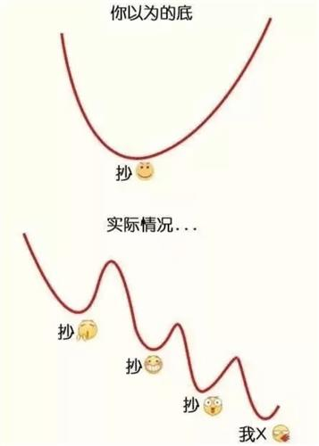
Investors want to buy at the low point and sell at the high point.

10 yuan to buy, 100 yuan to sell, earn a price difference, earn 90.

The essence of this problem is: buy low and sell high.

But the reality is often cruel.

When to buy and when to sell. In quantitative trading, there is an indicator, the relative strength of resistance support, namely RSRS.

To understand the relative strength of resistance support, we must first know what is resistance level and support level.

Resistance level refers to the pressure that may be encountered when the target price rises, that is, the traders believe that the seller's strength begins to surpass the buyer, so it is difficult for the price to continue to rise or fall from then on;

Support is the price at which traders believe that the buyer's power begins to surpass the seller, so as to stop falling or rebound.

The relative strength of resistance support is a way of using resistance level and support level. It no longer regards resistance level and support level as a fixed value, but as a variable, reflecting the traders' expected judgment on the top and bottom of the current market state.

We illustrate the application logic of the relative strength of support resistance according to different market conditions:

The market is in a rising bull market:

• If support is significantly stronger than resistance, the bull market will continue and prices will accelerate
• If resistance is significantly stronger than support, the bull market may be coming to an end and prices will peak

The market is in shock:

• If support is significantly stronger than resistance, the bull market may be about to start
• If resistance is significantly stronger than support, a bear market may be about to start

The market is in a downward bear market:

• If the support is obviously stronger than the resistance, the bear market may be coming to an end and the price will bottom out
• If the resistance is obviously stronger than the support, the bear market will continue and the price will fall faster

The daily maximum price and minimum price are a kind of resistance and support level, which is recognized by the trading behavior of all market participants on that day. A natural idea is to establish a linear regression between the highest price and the lowest price, and calculate the slope. Namely:

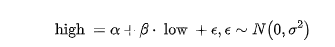
When the slope value is large, the support strength is greater than the resistance strength. In the bull market, the resistance is getting smaller and the upward space is large; In the bear market, the support is getting stronger and stronger, and the downward momentum is about to stop.

When the slope value is very small, the resistance strength is greater than the support strength. In the bull market, the resistance is getting stronger and the rising momentum is gradually stopped; In the bear market, the support is gradually sent, and the downward space is gradually larger.

There are two methods to calculate the RSRS index. The first method is to directly take the slope as the index value, and the second method is to standardize on the basis of the slope.

Taking the second method as an example, the timing strategy of RSRS slope standard sub index is as follows:

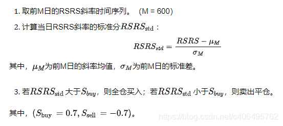
Small trial ox knife

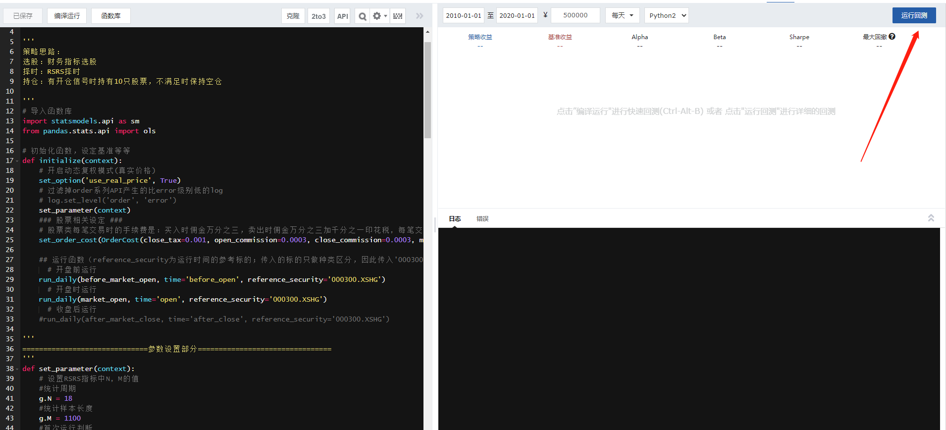
OK, which stock to buy, when to buy and when to sell. After these two problems are solved, we can start writing code.

Here you need to master the usage of poly width and some APIs.

This part is relatively simple, just direct to the official Manual of the platform.

Write the following code:

'''
Strategic thinking:
Stock selection: financial index stock selection
 Timing: RSRS Timing
 Position: hold 10 stocks when there is a position opening signal, and keep a short position when not satisfied

'''
# Import function library
import statsmodels.api as sm
from pandas.stats.api import ols

# Initialize functions, set benchmarks, etc
def initialize(context):
    # Enable dynamic reversion mode (real price)
    set_option('use_real_price', True)
    # Filter out the log s generated by the order series API that are lower than the error level
    # log.set_level('order', 'error')
    set_parameter(context)
    ### Stock related settings ###
    # The handling fee for each transaction of stocks is: 0.03% of the commission when buying, 0.03% of the commission when selling and 1 / 1000 of the stamp duty. The minimum commission for each transaction is 5 yuan
    set_order_cost(OrderCost(close_tax=0.001, open_commission=0.0003, close_commission=0.0003, min_commission=5), type='stock')
    
    ## Run function (reference_security is the reference target of the run time; the passed in target is only differentiated by type, so the passed in '000300.XSHG' or '510300.XSHG' is the same)
      # Operation before opening
    run_daily(before_market_open, time='before_open', reference_security='000300.XSHG') 
      # Operation at opening
    run_daily(market_open, time='open', reference_security='000300.XSHG')
      # Run after closing
    #run_daily(after_market_close, time='after_close', reference_security='000300.XSHG')
    
'''
==============================Parameter setting part================================
'''
def set_parameter(context):
    # Set the values of N and m in the RSRS index
    #Statistical cycle
    g.N = 18
    #Statistical sample length
    g.M = 1100
    #First run judgment
    g.init = True
    #Number of shares held
    g.stock_num = 10
    #Risk reference benchmark
    g.security = '000300.XSHG'
    # Set policy operation benchmark
    set_benchmark(g.security)
    #Record policy run days
    g.days = 0
    #set_benchmark(g.stock)
    # Buying threshold
    g.buy = 0.7
    g.sell = -0.7
    #It is used to record the beta value after regression, i.e. slope
    g.ans = []
    #It is used to calculate the beta value after weighted correction of the determined coefficient
    g.ans_rightdev= []
    
    # Calculate the RSRS slope index from January 5, 2005 to the start date of back test
    prices = get_price(g.security, '2005-01-05', context.previous_date, '1d', ['high', 'low'])
    highs = prices.high
    lows = prices.low
    g.ans = []
    for i in range(len(highs))[g.N:]:
        data_high = highs.iloc[i-g.N+1:i+1]
        data_low = lows.iloc[i-g.N+1:i+1]
        X = sm.add_constant(data_low)
        model = sm.OLS(data_high,X)
        results = model.fit()
        g.ans.append(results.params[1])
        #Calculate r2
        g.ans_rightdev.append(results.rsquared)
    
## Run function before opening     
def before_market_open(context):
    # Output run time
    #log.info('function run time (before_market_open): '+ str(context.current_dt.time()))
    g.days += 1
    # Send a message to wechat (add a simulated transaction and bind wechat to take effect)
    send_message('The policy runs normally%s day~'%g.days)

## Run function at opening
def market_open(context):
    security = g.security
    # Fill in the RSRS slope value of each date
    beta=0
    r2=0
    if g.init:
        g.init = False
    else:
        #RSRS slope index definition
        prices = attribute_history(security, g.N, '1d', ['high', 'low'])
        highs = prices.high
        lows = prices.low
        X = sm.add_constant(lows)
        model = sm.OLS(highs, X)
        beta = model.fit().params[1]
        g.ans.append(beta)
        #Calculate r2
        r2=model.fit().rsquared
        g.ans_rightdev.append(r2)
    
    # Calculate standardized RSRS index
    # Calculate mean series    
    section = g.ans[-g.M:]
    # Calculate mean series
    mu = np.mean(section)
    # Calculate standardized RSRS index sequence
    sigma = np.std(section)
    zscore = (section[-1]-mu)/sigma  
    #Calculate right deviation RSRS standard score
    zscore_rightdev= zscore*beta*r2
    
    # If the RSRS slope at the last time point is greater than the buying threshold, the whole position will buy
    if zscore_rightdev > g.buy:
        # Record this purchase
        log.info("The market risk is within a reasonable range")
        #Meet the conditions to run the transaction
        trade_func(context)
    # If the RSRS slope at the last time point is less than the sell threshold, the short position is sold
    elif (zscore_rightdev < g.sell) and (len(context.portfolio.positions.keys()) > 0):
        # Record this sale
        log.info("The market risk is too high and the short position is maintained")
        # Sell all stocks so that the final holding of this stock is 0
        for s in context.portfolio.positions.keys():
            order_target(s, 0)
            
#Strategic stock selection and trading    
def trade_func(context):
    #Get stock pool
    df = get_fundamentals(query(valuation.code,valuation.pb_ratio,indicator.roe))
    #Filter for Pb and roe greater than 0
    df = df[(df['roe']>0) & (df['pb_ratio']>0)].sort('pb_ratio')
    #Take stock noun as index
    df.index = df['code'].values
    #Take the reciprocal of roe
    df['1/roe'] = 1/df['roe']
    #Obtain comprehensive score
    df['point'] = df[['pb_ratio','1/roe']].rank().T.apply(f_sum)
    #Sort by score and take the specified number of shares
    df = df.sort('point')[:g.stock_num]
    pool = df.index
    log.info('Total selection%s Only stock'%len(pool))
    #Get the funds that should be allocated to each stock
    cash = context.portfolio.total_value/len(pool)
    #Get the list of positions already held
    hold_stock = context.portfolio.positions.keys() 
    #Sell stocks not in position
    for s in hold_stock:
        if s not in pool:
            order_target(s,0)
    #Buy stock
    for s in pool:
        order_target_value(s,cash)
#Scoring tool
def f_sum(x):
    return sum(x)
        
## Run function after closing  
def after_market_close(context):
    #Get all transaction records of the day
    trades = get_trades()
    for _trade in trades.values():
        log.info('Transaction record:'+str(_trade))
    #Print account total assets
    log.info('Total assets of today's account:%s'%round(context.portfolio.total_value,2))
    #log.info('##############################################################')

Write the code on the left and enter the back test time and amount.

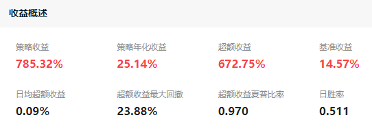
I directly back tested the effect from January 2010 to January 2020, and the ten-year return on Investment:

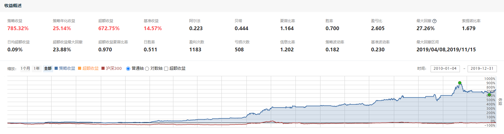
Direct take-off, initial capital of 500000, earned millions, very stable!

I retested the income of one and a half years from January 2020 to June 2021:

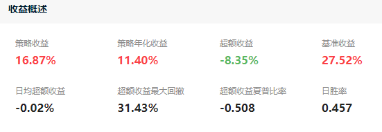
It lost 8.35% of the market, but it didn't lose. The annualized rate can also be 11.40%.

summary

This strategy does not use historical data and makes decisions according to some current indicators.

We still need to learn about investment and financial management. It's also good not to invest in the stock market and buy a bank regularly.

We study hard in the cold window. On the one hand, we want to achieve something, make money and live a comfortable life.

Schools teach us all kinds of basic knowledge, but rarely directly teach us how to make money, manage money and manage our own wealth.

So, teach yourself. Life is a toss, all kinds of knowledge to learn, very good, very interesting.

Now, although the stock market is a difficult model, there are still many opportunities. We can also use this time to supplement our knowledge.

This issue of hard core, like friends, forward, like a wave, let me see.

Interested, continue later.

I'm Jack. I'll see you next time!