preface
Study Xiaobai deeply. I hope you guys will forgive me if you make mistakes.
1, Data set loading and data set preprocessing
The data set can be downloaded directly from the Internet. Here, the data set is divided into training set and test set, but more often, we will be divided into training set, cross validation set and test set, so the training effect will be better.
(x, y), (x_test, y_test) = datasets.fashion_mnist.load_data()
X, y, X here_ test , y_ Test is of Numpy type and should be converted to tensor type
def preprocess(x, y):
    # And normalized
    x = tf.cast(x, dtype=tf.float32) / 255.
    y = tf.cast(y, dtype=tf.int32)
    return x, y
This function is used in combination with map() and passed into preprocess to complete mapping and type conversion
Then, in order to speed up the calculation, the whole sample is sliced into small samples of batch size
To facilitate operation, you can create an object of the dataset class, and then use the dataset member method batch
db = tf.data.Dataset.from_tensor_slices((x, y))
db = db.map(preprocess).shuffle(10000).batch(batches)
Do the same for the test set
Cycle through each batch data sample
sample = next(iter(db))
2, Construction of fully connected network layer
Use the Sequential container to generate an instance of the Sequential class
model = Sequential([
    # [b,784] @ [784,256]--> [b,256]
    layers.Dense(256, activation=tf.nn.relu),
    # [b,256]--> [b,128]
    layers.Dense(128, activation=tf.nn.relu),
    # [b, 128] --> [b,64]
    layers.Dense(64, activation=tf.nn.relu),
    # [b,64] --> [b,32]
    layers.Dense(32, activation=tf.nn.relu),
    # [b, 32] -- > [b, 10] output layer
    layers.Dense(10)
])
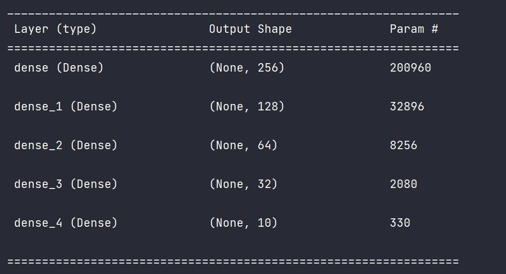
The initialization of network weights, offsets and input dimensions and the output of network model parameters are completed by member function build and summary
model.build(input_shape=[None, 28 * 28])
model.summary()
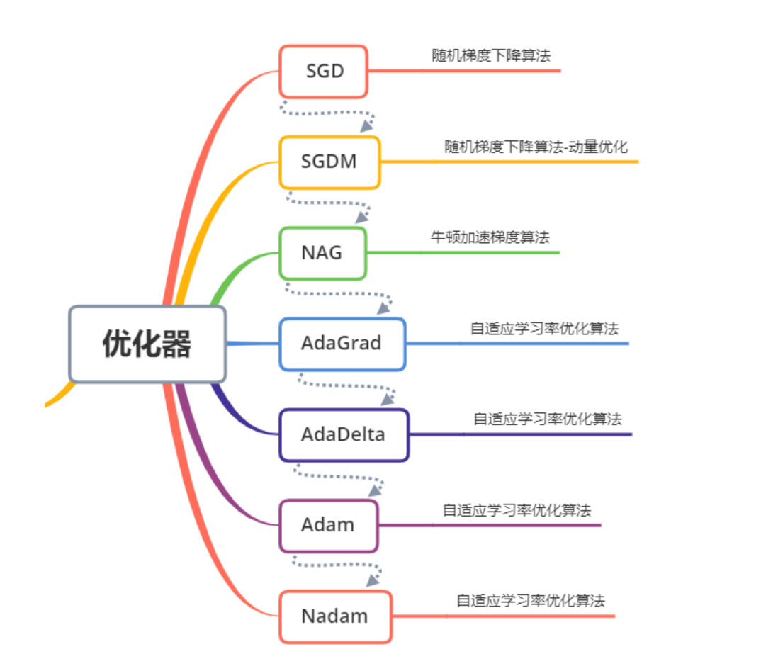
Construct optimizer
The optimizer mainly uses apply_gradients method passes in variables and corresponding gradients to iterate the given variables, or directly use the minimize method to iterate and optimize the objective function.

optimizers = optimizers.Adam(learning_rate=1e-3)
3, Calculate the gradient and cost function and update the parameters
When using the automatic derivation function to calculate the gradient, the forward calculation process needs to be placed in TF In the GradientTape () environment, the gradient() method of GradientTape object is used to automatically solve the gradient of parameters, and the optimizers object is used to update parameters
 with tf.GradientTape() as tape:
 	logits = model(x)
 	y_onehot = tf.one_hot(y, depth=10)
 	loss_ce = tf.losses.categorical_crossentropy(y_onehot, logits, from_logits=True)
    loss_ce = tf.reduce_mean(loss_ce)

grads = tape.gradient(loss_ce, model.trainable_variables)
optimizers.apply_gradients(zip(grads, model.trainable_variables))
4, Complete program
# -*- codeing = utf-8 -*-
# @Time : 10:02
# @Author:Paranipd
# @File : mnist_test.py
# @Software:PyCharm

import os
import tensorflow as tf
from tensorflow import keras
from tensorflow.keras import datasets, layers, optimizers, Sequential, metrics  # Data set, network layer, classifier, container

os.environ['TF_CPP_MIN_LOG_LEVEL'] = '2'  # Remove unnecessary error reports

# Preprocessing, parameter type conversion, and the loaded dataset is of Nunpy type
def preprocess(x, y):
    # And normalized
    x = tf.cast(x, dtype=tf.float32) / 255.
    y = tf.cast(y, dtype=tf.int32)
    return x, y

# Loading data set = training set + test set x,y: normal data type (Numpy)
# x.sahpe : (60000, 28 , 28) y.shape:(60000,)
# x.min-max:(0,255)   y :[0,9]
(x, y), (x_test, y_test) = datasets.fashion_mnist.load_data()
print(x.shape, x.dtype, y.shape, y.dtype)

# Number of batch samples
batches = 128
# Create a dataset whose elements are slices of a given tensor
# By using TF data. Interface provided by dataset from_tensor_slices will (x, y) - > the object of the dataset class
db = tf.data.Dataset.from_tensor_slices((x, y))
# map data type conversion
# shuffle randomly scatters the data set
# Batch forms multiple samples into a batch to speed up the calculation
# Note that different orders will have different results
db = db.map(preprocess).shuffle(10000).batch(batches)  # In order to make the number of data samples taken each time as batches
# print('db:', db)


db_test = tf.data.Dataset.from_tensor_slices((x_test, y_test))
db_test = db_test.map(preprocess).batch(batches)

# Iterate through the object db of the Dataset to obtain the next batch batch = = > sample = next (ITER (db))
db_iter = iter(db)
sample = next(db_iter)
print('batch:', sample[0].shape, sample[1].shape)

# Encapsulate a large network class object through Sequential container
model = Sequential([
    # [b,784] @ [784,256]--> [b,256]
    layers.Dense(256, activation=tf.nn.relu),
    # [b,256]--> [b,128]
    layers.Dense(128, activation=tf.nn.relu),
    # [b, 128] --> [b,64]
    layers.Dense(64, activation=tf.nn.relu),
    # [b,64] --> [b,32]
    layers.Dense(32, activation=tf.nn.relu),
    # [b, 32] -- > [b, 10] output layer
    layers.Dense(10)
])

# Initialize the weights and dimensions of the network
model.build(input_shape=[None, 28 * 28])    # Class method of Sequential class
# Output the parameter status of each layer of the network mode and view the structure of the network model
model.summary()

# w = w - lr * grad
# Setting of learning rate and updating parameters
optimizers = optimizers.Adam(learning_rate=1e-3)


def main():
    # Iterate the entire dataset 30 times
    for epoch in range(30):
        # Iterate over the data set object, wait for the step parameter, and complete a batch of data training, which is called a step
        # Partial data sets are processed in batches, and 128 samples are processed at a time
        for step, (x, y) in enumerate(db):
            # x: [b, 28,28] = = > [b, 784] one dimensional
            # y: [b]
            x = tf.reshape(x, [-1, 28 * 28])

            # When using the automatic derivation function to calculate the gradient, the forward calculation process needs to be placed in TF Gradienttape() environment
            # The gradient() method of GradientTape object is used to automatically solve the gradient of parameters
            # And use the optimizers object to update the parameters
            with tf.GradientTape() as tape:    # Gradient recorder
                # [b,784] ==> [b,10]
                # model(x) is actually in the calling class__ call__ method
                # Output network model (forward calculation) results
                logits = model(x)
                # onehot coding
                y_onehot = tf.one_hot(y, depth=10)

                # Mean square deviation cost function
                loss_mse = tf.reduce_mean(tf.losses.MSE(y_onehot, logits))
                # Cross entropy loss calculation function
                loss_ce = tf.losses.categorical_crossentropy(y_onehot, logits, from_logits=True)
                loss_ce = tf.reduce_mean(loss_ce)

            # Derivation of all optimizable variables
            grads = tape.gradient(loss_ce, model.trainable_variables)
            # Updating can optimize the tensor
            # zip packages the corresponding elements into tuples, which form a list
            optimizers.apply_gradients(zip(grads, model.trainable_variables))

            if step % 100 == 0:
                print(epoch, step, 'loss:', float(loss_ce), float(loss_mse))

        # test calculates an accuracy
        total_correct = 0
        total_num = 0
        for x, y in db_test:
            # x: [b,28,28] ==> [b,784]
            # y: [b]
            x = tf.reshape(x, [-1, 28 * 28])
            # [b,10]
            logits = model(x)
            # logits --> prob: [b,10] int64

            # Normalize the output results to obtain the probability that the sum is 1
            prob = tf.nn.softmax(logits, axis=1)  # [0,1]
            # Find the index position corresponding to the maximum value of the dimension
            pred = tf.argmax(prob, axis=1)
            pred = tf.cast(pred, dtype=tf.int32)
            # pred:[b]
            # y: [b]
            # correct: [b], True(1): equal; False(0): not equal
            correct = tf.equal(pred, y)
            correct = tf.reduce_sum(tf.cast(correct, dtype=tf.int32))
            # Number of forecast pairs
            total_correct += int(correct)
            # Total quantity
            total_num += x.shape[0]
        # accuracy
        acc = total_correct / total_num
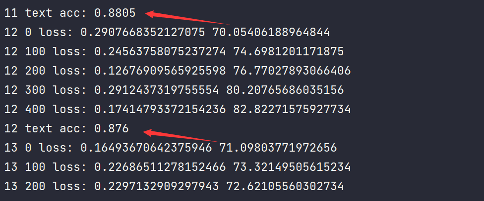
        print(epoch, 'text acc:', acc)

if __name__ == "__main__":
    main()
Model results


The final prediction accuracy is about 0.87. If we do some optimization and error processing, the accuracy can be higher.
summary
Tip: here is a summary of the article: