1. CIFAR-10

Cifar-10 is a data set collected by Alex Krizhevsky and Ilya Sutskever, two disciples of Hinton, for universal object recognition. Cifar is an advanced science project institute led by the Canadian government. Hinton, Bengio and his students received a small amount of money from Cifar in 2004 to build neurocomputing and adaptive perception projects. This project brings together many computer scientists, biologists, electrical engineers, neuroscientists, physicists and psychologists to accelerate the process of Deep Learning. From this lineup, DL The data mining of ML system is far away. Deep Learning emphasizes adaptive perception and artificiality Intelligence Data Mining emphasizes high speed. Big data Statistical mathematical analysis is the intersection of computer and mathematics.

Cifar-10 is composed of 60,000 32*32 RGB color images, totaling 10 categories. 50,000 exercises, 10,000 exercises test (Cross-validation). The greatest feature of this data set is that it migrates recognition to universal objects and applies it to multi-classification (sisterly data set Cifar-100 reaches 100 categories, ILSVRC competition is 1000 categories).

It can be seen that compared with mature face recognition, universal object recognition is a huge challenge. There are a lot of features and noises in the data, and the proportion of recognizing objects is different. Therefore, Cifar-10 is quite challenging compared with the traditional image recognition data set. For more information, please refer to CIFAR-10 page And Alex Krizhevsky's Technical Report.

2. Model

In previous blog posts, we have used TensorFlow to build a simple MNIST model for handwritten numeral recognition, mainly referring to Yann LeCun's paper published in 1998. Gradient-Based Learning Applied to Document Recognition The classical LeNet5 network proposed in this paper:

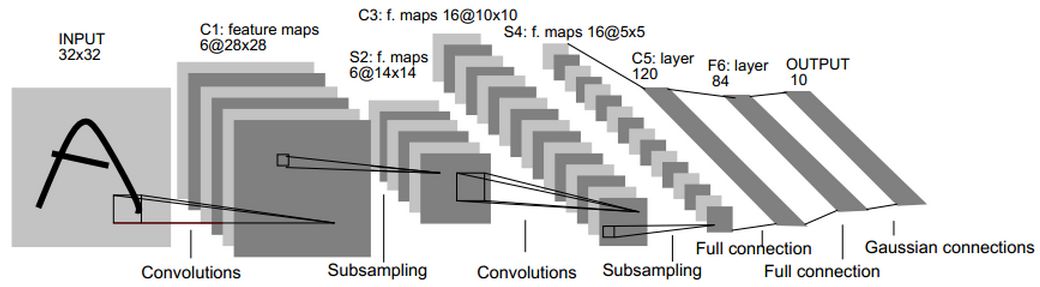
The network consists of convolution layer, pooling layer and full connection layer. The parameters are trained by gradient descent method. However, in the face of the complex problem of universal object classification, the network structure has been far from meeting the needs.

In this blog, we will analyze the improved techniques of AlexNet network for the classification of pervasive objects, which prevent model over-fitting and enhance the normalization ability.

• Data Augmentation is used for image flipping and random clipping.
• Local response normalization (LRN) is used behind the convolution-maximum pooling layer.
• Modified linear activation (ReLu), Dropout and overlapping Pooling were used.

As well as the implementation of TensorFlow code on CIFAR-10, we add pre-access queues for input data, visualization of network behavior, maintenance of sliding mean of parameters, setting learning rate decreases with iteration, and finally add L2 regular training to Losses to improve the training speed and recognition rate of the network.

The code results and network structure used in this article are as follows:

file	Explain
cifar10_input.py	Read the contents of the local CIFAR-10 binary file format
cifar10.py	Establishment of CIFAR-10 Model
cifar10_train.py	Training CIFAR-10 Model on CPU or GPU
cifar10_multi_gpu_train.py	The CIFAR-10 model is trained on multiple GPU s.
cifar10_eval.py	Evaluating the predictive performance of CIFAR-10 model

Multiple GPU versions of the model are provided in the reference code, but only CPU is used in this article.

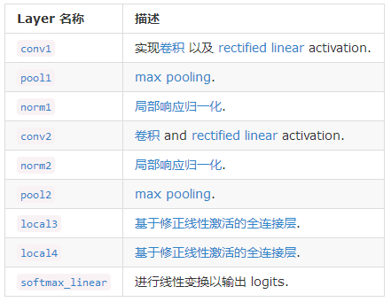
3. Network Structure

The code of CIFAR-10 network model is located in cifar10.py. The complete training diagram contains about 765 operations. The following modules are used to construct training maps to maximize code reuse:

• Model input: including inputs(), distorted_inputs() and other operations, which are used to read CIFAR-10 images and preprocess them, respectively, as input for subsequent evaluation and training;
• Model prediction: some operations, such as inference(), are used for statistical calculation, such as classifying the images provided;
• Model training: Some operations including loss() and train() are used to calculate losses, calculate gradients, update variables and present final results.

3.1 Model Input

The input model is established by cifar10_input.inputs() and cifar10_input.distorted_inputs() functions, which read image files from CIFAR-10 binary files. The implementation is defined in cifar10_input.py and the data used is CIFAR-10 page The following 162M binary file can use the tf.FixedLengthRecordReader function because the number of bytes stored in each image is fixed.

After loading the image data, the data is augmented through the following processes:

1. Uniform clipping to 24x24 pixel size, clipping the central area for evaluation or random clipping for training;
2. Random left-right flip of the image;
3. Random transform image brightness;
4. Random transform image contrast;
5. The picture will be whitened approximately.

Among them, whitening processing or standardization processing is to subtract the mean value of image data, divide by variance, ensure zero mean value of data, variance is 1, so as to reduce the redundancy of input image, remove the correlation between input features as far as possible, and make the network insensitive to the dynamic range change of image. A principle of mean file in Cafe.

View all available transformations in the list of Images pages, and add tf.summary.image for each original graph to facilitate viewing in Tensor Board:

Loading images from disk and transforming them takes a lot of processing time. To avoid these operations slowing down the training process, these operations are performed in parallel with 16 separate threads, which are sequentially arranged in a TensorFlow queue and returned to the pre-processed encapsulated tensor. Each execution generates a batch_size sample [images, labels]. The test data is generated by cifar10_input.inputs() function. The test data does not need to flip or modify the brightness and contrast of the picture. It needs to cut the 24*24 block in the middle of the picture and standardize the data.  

The main functions are used as follows:

1. maybe_download_and_extract():              #Download and decompress data  
2. distorted_inputs(data_dir, batch_size):    #Read in data and increase data  
3.     read_cifar10(filename_queue):      #Read binary data  
4.     tf.random_crop();                  #Random clipping, old version tf.image.random_crop  
5.     tf.image.random_flip_left_right(); #Turn left and right  
6.     tf.image.random_brightness();      #Transform the brightness of the image  
7.     tf.image.random_contrast();        #Contrast of transformed images  
8.     tf.image.per_image_standardization(); #Standardize the image, the old version is tf.image.per_image_whitening  
9.     _generate_image_and_label_batch();    #Using tf.train.shuffle_batch() to create multiple threads to build batch from tensor queues  

3.2 Model Prediction

The prediction process of the model is constructed by inference(), input is images and output is logits of the last layer.

Before building the model, we construct the weight constructor _variable_with_weight_decay(name, shape, stddev, wd), where WD is used to add L2 regularization to losses, which can prevent over-fitting and improve generalization ability:

1. def _variable_with_weight_decay(name, shape, stddev, wd):  
2.   var = _variable_on_cpu(name, shape,  
3.                          tf.truncated_normal_initializer(stddev=stddev))  
4.   if wd:  
5.     weight_decay = tf.multiply(tf.nn.l2_loss(var), wd, name='weight_loss')  
6.     tf.add_to_collection('losses', weight_decay)  
7.   return var  

Then we start to build a network, the weight of the first convolution layer does not carry out L2 regularization, so the kernel(wd) item is set to 0, and the biases with a value of 0 are established. The results of conv1 are activated by ReLu and summarized by _activation_summary(); then the first pooling layer is established, and the inconsistency of maximum pooling size and step size can increase the richness of data; finally, the LRN layer is established.( The LRN layer imitates the "lateral inhibition" mechanism of the biological nervous system to create a competitive environment for the activities of local neurons, which makes the larger response value become relatively larger, and inhibits other neurons with smaller feedback, thus enhancing the generalization ability of the model. Relu, an activation function with no upper bound, is useful because it can select larger feedback from the response of multiple convolution cores nearby, but it is not suitable for sigmoid, which has fixed boundaries and can suppress excessive activation function.

1. # conv1  
2.   with tf.variable_scope('conv1') as scope:  
3.     kernel = _variable_with_weight_decay('weights', shape=[5, 5, 3, 64],  
4.                                          stddev=1e-4, wd=0.0)  
5.     conv = tf.nn.conv2d(images, kernel, [1, 1, 1, 1], padding='SAME')  
6.     biases = _variable_on_cpu('biases', [64], tf.constant_initializer(0.0))  
7.     bias = tf.nn.bias_add(conv, biases)  
8.     conv1 = tf.nn.relu(bias, name=scope.name)  
9.     _activation_summary(conv1)  
10.   
11.   # pool1  
12.   pool1 = tf.nn.max_pool(conv1, ksize=[1, 3, 3, 1], strides=[1, 2, 2, 1],  
13.                          padding='SAME', name='pool1')  
14.   # norm1  
15.   norm1 = tf.nn.lrn(pool1, 4, bias=1.0, alpha=0.001 / 9.0, beta=0.75,  
16.                     name='norm1')  

In the second layer and the first layer, besides the change of input parameters, the biases values are all initialized to 0.1. The order of maximum pooling and LRN layer is changed. First, LRN is carried out, and then the maximum pooling layer is used.

1. # conv2  
2.   with tf.variable_scope('conv2') as scope:  
3.     kernel = _variable_with_weight_decay('weights', shape=[5, 5, 64, 64],  
4.                                          stddev=1e-4, wd=0.0)  
5.     conv = tf.nn.conv2d(norm1, kernel, [1, 1, 1, 1], padding='SAME')  
6.     biases = _variable_on_cpu('biases', [64], tf.constant_initializer(0.1))  
7.     bias = tf.nn.bias_add(conv, biases)  
8.     conv2 = tf.nn.relu(bias, name=scope.name)  
9.     _activation_summary(conv2)  
10.   
11.   # norm2  
12.   norm2 = tf.nn.lrn(conv2, 4, bias=1.0, alpha=0.001 / 9.0, beta=0.75,  
13.                     name='norm2')  
14.   # pool2  
15.   pool2 = tf.nn.max_pool(norm2, ksize=[1, 3, 3, 1],  
16.                          strides=[1, 2, 2, 1], padding='SAME', name='pool2')  

In the third layer, we need to flatten all the output results of the previous convolution layer, change each sample into a one-dimensional vector using tf.reshape function, get_shape function to get the length of flattened data, and initialize weights and biases of the whole connection layer. In order to prevent over-fitting of the whole connection layer, we set a non-zero wd value of 0.004. Let all the parameters of this layer be constrained by the L2 regularity, and still use it. The Relu activation function is nonlinearized. Similarly, the fourth full connection layer can be established.

1. # local3  
2.   with tf.variable_scope('local3') as scope:  
3.     # Move everything into depth so we can perform a single matrix multiply.  
4.       
5.     reshape = tf.reshape(pool2, [FLAGS.batch_size, -1])  
6.     dim = reshape.get_shape()[1].value   
7.       
8.   
9.     weights = _variable_with_weight_decay('weights', shape=[dim, 384],  
10.                                           stddev=0.04, wd=0.004)  
11.     biases = _variable_on_cpu('biases', [384], tf.constant_initializer(0.1))  
12.     local3 = tf.nn.relu(tf.matmul(reshape, weights) + biases, name=scope.name)  
13.     _activation_summary(local3)  

At the end of the software max_linear layer, create weights and biases for this layer without adding L2 regularization. In this model, unlike the previous example, sotfmax is used to output the final result, because the operation of softmax is placed in the part of calculating loss, and the linear return value logits and labels are used to calculate loss, which will be described in the next blog post.

1. # softmax, i.e. softmax(WX + b)  
2.   with tf.variable_scope('softmax_linear') as scope:  
3.     weights = _variable_with_weight_decay('weights', [192, NUM_CLASSES],  
4.                                           stddev=1/192.0, wd=0.0)  
5.     biases = _variable_on_cpu('biases', [NUM_CLASSES],  
6.                               tf.constant_initializer(0.0))  
7.     softmax_linear = tf.add(tf.matmul(local4, weights), biases, name=scope.name)  
8.     _activation_summary(softmax_linear)  
9.   
10.   return softmax_linear  

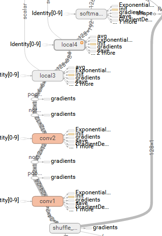
At this point, the inference of the entire network has been built, and the structure can be viewed with Tensor Board:

3.3 Loss Function

We recall the previous method of calculating loss using cross entropy:

1. y_conv = tf.nn.softmax(tf.matmul(h_fc1_drop,W_fc2) + b_fc2)  
2. cross_entropy = tf.reduce_sum(-y_*tf.log(y_conv))  

Here y_conv is the logits value after tf.nn.softmax (the probability value belonging to each category), shape is [batch_size, num_classes], the sum of logit vector elements of each sample is 1; y_is the labels value after one hot encoding, shape is [batch_size, num_classes], only one label element in each sample is 1, the rest is 0. In later versions, TensorFlow provides a more convenient API that combines software Max and cross entropy. Calculations:

1. cross_entropy_loss = tf.nn.softmax_cross_entropy_with_logits(labels=y_, logits=y_conv)    

In CIFAR-10, the shape of labels is [batch_size], and the label of each sample is a number of 0 to 9, representing 10 classes. These classes are mutually exclusive, and each class is mutually exclusive. CIFAR-10 pictures can only be labeled as the only label: a picture may be a dog or a truck, not both. So we need one hot encoding for label value. The transformation process is tedious. The new version of TensorFlow API supports sparse_to_dense for unique labels. It only takes one step:

1. cross_entropy_loss = tf.nn.sparse_softmax_cross_entropy_with_logits(logits=logits, labels=labels, name='cross_entropy_pre_example')  

The shape of labels here is [batch_size, 1]. Then use tf.add_to_collection to add cross entropy's loss to the overall losses collection. Finally, tf.add_n is used to sum all the loss in the collection of the overall losses to get the final loss. It also returns, which contains cross entropy loss and L2 loss of weight in the last two full connection layers.

1. tf.add_to_collection(name='losses', value=cross_entropy_loss)  
2. return tf.add_n(inputs=tf.get_collection(key='losses'), name='total_loss')  

3.4 Model Training
After defining loss, we need to define train() that accepts loss and returns train op.

Firstly, the learning rate is defined, and it decreases with the number of iterations, and summary:

1. lr = tf.train.exponential_decay(INITIAL_LEARNING_RATE, global_step, decay_steps, LEARNING_RATE_DECAY_FACTOR, staircase=True)  
2. tf.summary.scalar('learning_rate', lr)  

In addition, we generate sliding mean and aggregation for loss, and maintain the sliding average of variables (Moving Average) by using exponential decay. When training the model, it is beneficial to maintain the sliding mean of training parameters. Using sliding parameters in the testing process will improve the actual performance of the model, that is, the accuracy. apply() The method adds shadow copies of trained variables, and adds operations to maintain the sliding mean of variables to shadow copies. The average() method can access shadow variables, which is very useful in creating evaluation model s. The sliding mean is calculated by exponential decay. The initial value of shadow variable is the same as that of trained variables. The updated formula is shadow_variable = decay * shadow_variable + (1 - decay). * variable.

1. _add_loss_summaries(total_loss):  
2.   #Create a new exponential sliding average object  
3.   loss_averages = tf.train.ExponentialMovingAverage(0.9, name='avg')  
4.   #Return all variables corresponding to the keyword'losses'from the dictionary set, including cross-entropy loss and regularization loss  
5.   losses = tf.get_collection('losses')  
6.   #Create'shadow variables'and add operations to maintain sliding averages  
7.   loss_averages_op = loss_averages.apply(losses + [total_loss])  
8.   
9.   # Attach a scalar summary to all individual losses and the total loss; do the  
10.   # same for the averaged version of the losses.  
11.   for l in losses + [total_loss]:  
12.     # Name each loss as '(raw)' and name the moving average version of the loss  
13.     # as the original loss name.  
14.     tf.summary.scalar(l.op.name +' (raw)', l)  
15.     tf.summary.scalar(l.op.name, loss_averages.average(l))  
16.   
17.   return loss_averages_op  

Then, we define the training methods and objectives. tf.control_dependencies is a context manager, which controls the execution order of nodes. First, we execute the operations in [] and then the operations in context:

1. loss_averages_op = _add_loss_summaries(total_loss) #Updating of loss variables  
2. with tf.control_dependencies([loss_averages_op]):  
3.     opt = tf.train.GradientDescentOptimizer(lr)      
4.     grads = opt.compute_gradients(total_loss)      #Return calculated (gradient, variable) pairs  
5.    
6. #Return to one-step gradient update operation.  
7. apply_gradient_op = opt.apply_gradients(grads, global_step=global_step)   

Finally, the attenuation rate is dynamically adjusted to return the sliding update operation of the model parameter variables, namely train op:

1. variable_averages = tf.train.ExponentialMovingAverage(  
2.       MOVING_AVERAGE_DECAY, global_step)  
3. variables_averages_op = variable_averages.apply(tf.trainable_variables())  
4.   
5. with tf.control_dependencies([apply_gradient_op, variables_averages_op]):  
6.     train_op = tf.no_op(name='train')  
7.   
8. return train_op  

4. Training process

The above steps complete the definition of data input, model prediction, loss and training, and then call in turn to establish the training and summary process:

1. def train():  
2.   """Train CIFAR-10 for a number of steps."""  
3.   #Specify the current graph as the default graph  
4.   with tf.Graph().as_default():  
5.     #Setting trainable=False prevents sliding updates to global_step variables during training  
6.     global_step = tf.Variable(0, trainable=False)  
7.   
8.     # Get images and labels for CIFAR-10.  
9.     #Preprocessing of input image, including brightness, contrast, image flip, etc.  
10.     images, labels = cifar10.distorted_inputs()  
11.   
12.     # Build a Graph that computes the logits predictions from the  
13.     # inference model.  
14.     logits = cifar10.inference(images)  
15.   
16.     # Calculate loss.  
17.     loss = cifar10.loss(logits, labels)  
18.   
19.     # Build a Graph that trains the model with one batch of examples and  
20.     # updates the model parameters.  
21.     train_op = cifar10.train(loss, global_step)  
22.   
23.     #Create a saver object to save parameters to a file  
24.     saver = tf.train.Saver(tf.global_variables())  
25.   
26.     #Returns the string type tensor of all summary objects after merge and serialize  
27.     summary_op = tf.summary.merge_all()  
28.   
29.     #The log_device_placement parameter can record the device used for each operation. There are many operations here, so it is set to False.  
30.     sess = tf.Session(config=tf.ConfigProto(  
31.         log_device_placement=FLAGS.log_device_placement))  
32.   
33.     #Variable initialization  
34.     init = tf.global_variables_initializer()  
35.     sess.run(init)  
36.   
37.     ckpt = tf.train.get_checkpoint_state(FLAGS.train_dir)  
38.     if ckpt and ckpt.model_checkpoint_path:  
39.       # Restores from checkpoint  
40.       saver.restore(sess, ckpt.model_checkpoint_path)  
41.       print ("restore from file")  
42.     else:  
43.       print('No checkpoint file found')  
44.   
45.     #Start all queuerunners  
46.     tf.train.start_queue_runners(sess=sess)  
47.   
48.     summary_writer = tf.summary.FileWriter(FLAGS.train_dir,  
49.                                             graph=sess.graph)  
50.   
51.     for step in xrange(FLAGS.max_steps):  
52.       start_time = time.time()  
53.       _, loss_value = sess.run([train_op, loss])  
54.       duration = time.time() - start_time  
55.         
56.       #To verify the reasonableness of loss_value calculated by the current iteration  
57.       assert not np.isnan(loss_value), 'Model diverged with loss = NaN'  
58.   
59.       if step % 10 == 0:  
60.         num_examples_per_step = FLAGS.batch_size  
61.         examples_per_sec = num_examples_per_step / duration  
62.         sec_per_batch = float(duration)  
63.   
64.         format_str = ('%s: step %d, loss = %.2f (%.1f examples/sec; %.3f '  
65.                       'sec/batch)')  
66.         print (format_str % (datetime.now(), step, loss_value,  
67.                              examples_per_sec, sec_per_batch))  
68.         
69.       if step % 100 == 0:  
70.         summary_str = sess.run(summary_op)  
71.         summary_writer.add_summary(summary_str, step)  
72.   
73.       # Save the model checkpoint periodically.  
74.       if step % 1000 == 0 or (step + 1) == FLAGS.max_steps:  
75.         checkpoint_path = os.path.join(FLAGS.train_dir, 'model.ckpt')  
76.         saver.save(sess, checkpoint_path, global_step=step)  

It's important to note that you must run start_queue_runners to start the previously mentioned thread for image data augmentation, which uses 16 threads for acceleration.

In the training process of each step, we need to use session run method to perform the calculation of images, labels, train_op and loss, record the time spent on each step, calculate and display the current loss every 10 steps, the number of training samples per second, and the time spent on training a batch data. It is more convenient to monitor the whole training process.

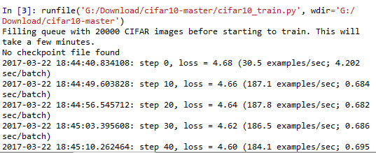
By executing scripts Python cifar10_train.py starts the training process. When any task is started on CIFAR-10 for the first time, the CIFAR-10 dataset will be downloaded automatically. The dataset is about 160M in size, and then output:

5. Model evaluation

cifar10_train.py periodically saves all the parameters in the model in the checkpoint file, but does not evaluate the model. cifar10_eval.py uses this checkpoint file on another part of the data set test Prediction performance. utilize The inference() function reconstructs the model and tests it with all 10,000 CIFAR-10 images in the evaluation data set. The final calculated accuracy is 1:N, N = the highest confidence item in the predicted value and the frequency matched with the real label of the picture. In order to monitor the improvement of the model in the training process, the script files used for evaluation will run periodically on the latest checkpoint files, which are generated by the cifar10_train.py mentioned above.

After running the cifar10_eval.py file, we can get output like this:

1. 2017-03-22 19:00:00.223784: precision @ 1 = 0.099  

The script only returns the precision @ 1 periodically, and the accuracy rate returned in this case is 9.9% due to the few iterations. cifar10_eval.py also returns some other brief information that can be visualized in TensorBoard, which can be used to further understand the model during the evaluation process.

Our training script calculates the Moving Average for all learning variables, and the evaluation script directly replaces all learning model parameters with corresponding sliding average, which can improve the performance of the model in the evaluation process.