The code of this article comes from natural language processing with TensorFlow, written by Thushan Ganegedara.
Yes, dear children, the official account of humbly Xiao Li has been opened and is looking forward to discussing with you.
0 Preface
The code of this article comes from natural language processing with TensorFlow, written by Thushan Ganegedara. Based on the author's code, I added some of my own comments (the author's comments are in English and my comments are in Chinese). The code has been uploaded to github, Here is the link.
If there are any mistakes or parts that are not explained clearly, please comment below and I will change them after seeing them.
For the principle of Word2Vec and two optimization methods - hierarchical softmax and negative sampling, if you have questions, please refer to my previous two articles: Detailed derivation of Word2Vec principle and formula,Word2Vec's Hierarchical Softmax and Negative Sampling.
TensorFlow version is 1.8.0.
1 data set preparation
There is nothing to say in the data set preparation section, that is, downloading data.
url = 'http://www.evanjones.ca/software/'

def maybe_download(filename, expected_bytes):
    """Download a file if not present, and make sure it's the right size."""
    if not os.path.exists(filename):
        print('Downloading file...')
        filename, _ = urlretrieve(url + filename, filename)
    statinfo = os.stat(filename)
    if statinfo.st_size == expected_bytes:
        print('Found and verified %s' % filename)
    else:
        print(statinfo.st_size)
        raise Exception(
          'Failed to verify ' + filename + '. Can you get to it with a browser?')
    return filename

filename = maybe_download('wikipedia2text-extracted.txt.bz2', 18377035)
But I don't know why. I open this website as Not found, but I can download data.
2 read data without preprocessing
def read_data(filename):
    """Extract the first file enclosed in a zip file as a list of words"""

    with bz2.BZ2File(filename) as f:
        data = []
        file_string = f.read().decode('utf-8')
        file_string = nltk.word_tokenize(file_string)
        data.extend(file_string)
    return data

words = read_data(filename)
print('Data size %d' % len(words))
print('Example words (start): ',words[:10])
print('Example words (end): ',words[-10:])
This step is to read the data from the downloaded file and do word segmentation. Since there are more than 10 million data without preprocessing, the running speed of this line of code is very slow. Moreover, the data that is not preprocessed is not used later.
The output is as follows:
Data size 11634727
Example words (start):  ['Propaganda', 'is', 'a', 'concerted', 'set', 'of', 'messages', 'aimed', 'at', 'influencing']
Example words (end):  ['useless', 'for', 'cultivation', '.', 'and', 'people', 'have', 'sex', 'there', '.']
3 read data and do preprocessing
def read_data(filename):
    """
    Extract the first file enclosed in a zip file as a list of words
    and pre-processes it using the nltk python library
    """

    with bz2.BZ2File(filename) as f:

        data = []
        file_size = os.stat(filename).st_size
        chunk_size = 1024 * 1024 # reading 1 MB at a time as the dataset is moderately large
        print('Reading data...')
        for i in range(ceil(file_size//chunk_size)+1):
            bytes_to_read = min(chunk_size,file_size-(i*chunk_size))
            file_string = f.read(bytes_to_read).decode('utf-8')
            file_string = file_string.lower()
            # tokenizes a string to words residing in a list
            file_string = nltk.word_tokenize(file_string)
            data.extend(file_string)
    return data

words = read_data(filename)
print('Data size %d' % len(words))
print('Example words (start): ',words[:10])
print('Example words (end): ',words[-10:])
This step of preprocessing is mainly in two parts. The first part is to read only 1M data at a time, and the second part is to change all words into lowercase.
The output is as follows:
Reading data...
Data size 3361192
Example words (start):  ['propaganda', 'is', 'a', 'concerted', 'set', 'of', 'messages', 'aimed', 'at', 'influencing']
Example words (end):  ['favorable', 'long-term', 'outcomes', 'for', 'around', 'half', 'of', 'those', 'diagnosed', 'with']
4 create dictionary
This step is mainly to map words and ID S. Take "I like to go to school" as an example. The mapping rules are as follows:
- dictionary: mapping relationship between words and ID S (e.g. {'I': 0, 'like': 1, 'to': 2, 'go': 3, 'school': 4}).
- reverse_ dictionary: mapping relationship between ID and words (i.e. reverse the key value of dictionary) (e.g. {0: 'I', 1: 'like', 2: 'to', 3: 'go', 4: 'school'}).
- count: a list. Each element in the list is a tuple. The elements in each tuple are words and frequencies (e.g. [('I', 1), (like ', 1), (to', 2), (go ', 1), (school', 1)]).
- data: words in the text, which are replaced by ID (e.g. [0, 1, 2, 3, 2, 4]).
- UNK: rare words, that is, all words after removing the 50000 words with the highest frequency.
# we restrict our vocabulary size to 50000
vocabulary_size = 50000

def build_dataset(words):
    count = [['UNK', -1]]  # Because the value of - 1 needs to be changed later, here is the list
    # Gets only the vocabulary_size most common words as the vocabulary
    # All the other words will be replaced with UNK token
    # That is to say, 50000 most common words are extracted, and the rest are classified as' UNK '
    count.extend(collections.Counter(words).most_common(vocabulary_size - 1))
    dictionary = dict()

    # Create an ID for each word by giving the current length of the dictionary
    # And adding that item to the dictionary
    # Word: word name,: Number of occurrences (frequency)
    # This step is to map words and IDS
    # dictionary: {'word1': 0, 'word2': 1, 'word3': 2, ...}
    for word, _ in count:
        dictionary[word] = len(dictionary)

    data = list()
    unk_count = 0  # How many Unks are recorded
    # Traverse through all the text we have and produce a list
    # where each element corresponds to the ID of the word found at that index
    # If the word is in a dictionary, the id of the word is used
    # Otherwise, it is UNK with id 0 (because the first word in the dictionary is also UNK)
    for word in words:
        # If word is in the dictionary use the word ID,
        # else use the ID of the special token "UNK"
        if word in dictionary:
            index = dictionary[word]
        else:
            index = 0  # dictionary['UNK']
            unk_count = unk_count + 1
        data.append(index)

    # update the count variable with the number of UNK occurences
    # Updating count is actually updating the number of Unks
    count[0][1] = unk_count

    reverse_dictionary = dict(zip(dictionary.values(), dictionary.keys()))
    # Make sure the dictionary is of size of the vocabulary
    assert len(dictionary) == vocabulary_size

    return data, count, dictionary, reverse_dictionary

data, count, dictionary, reverse_dictionary = build_dataset(words)
print('Most common words (+UNK)', count[:5])
print('Sample data', data[:10])
del words  # Hint to reduce memory.
First, let's talk about the count. In the above explanation, the elements in count are tuples, but build_ The first row of the dataset defines count = [['UNK', -1]]. This is because the value of - 1 needs to be changed later, so the count[0] defined here is a list. In other words, count is as follows:
count = [
		['UNK', 68751],
		('the', 226893),
		...
		('suggested', 336)
]
Then, the creation of dictionary is also very spiritual. First, extract the words in count (the words in count are arranged in order from large to small) and put them into the dictionary. Since count is generated through collections, there is no duplicate value. After putting it into the dictionary, the ID is the length of the dictionary. Since a key value pair will be put in each round, the length of the dictionary will be increased by 1 in each round. In this way, the ID will be increased by 1 at a time.
Then, extract the value in the dictionary and put it into data, and build reverse according to its key value_ dictionary.
The output is as follows:
Most common words (+UNK) [['UNK', 68751], ('the', 226893), (',', 184013), ('.', 120919), ('of', 116323)]
Sample data [1721, 9, 8, 16479, 223, 4, 5168, 4459, 26, 11597]
5. Define the batch of skip gram
Skip gram predicts the context of a word. Its network structure is as follows:
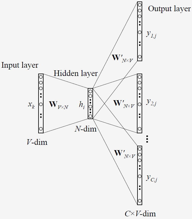
It should be noted here that the hidden layer of Word2Vec is linear, so there is no activation function in the hidden layer.
Because this step is to define the labels of input and output. Set batch as the input word; Labels is the context of the input word; Let span be the window size and target word, and the size is 2 ∗ w i n d o w _ s i z e + 1 2 * {\rm window\_size} + 1 2∗window_size+1, due to window_size is the window size of one side, so it should be multiplied by 2, that is, the context size is 2 ∗ w i n d o w _ s i z e 2 * {\rm window\_size} 2∗window_size.
data_index = 0

def generate_batch_skip_gram(batch_size, window_size):
    # data_index is updated by 1 everytime we read a data point
    # Call external variables
    global data_index
    # print('global data_index:', data_index)
    # print('batch_size:', batch_size)
    # print('window_size:', window_size)

    # two numpy arras to hold target words (batch)
    # and context words (labels)
    # Batch: the random initial size is batch_size  ×  Vector of 1
    # labels: the random initial size is 1 ×  batch_ Vector of size
    batch = np.ndarray(shape=(batch_size), dtype=np.int32)
    labels = np.ndarray(shape=(batch_size, 1), dtype=np.int32)

    # span defines the total window size, where
    # data we consider at an instance looks as follows.
    # [ skip_window target skip_window ]
    # span: 2 * window size + 1, i.e. left and right context + target word
    span = 2 * window_size + 1

    # The buffer holds the data contained within the span
    # The queue created by deque can add data from left to right
    buffer = collections.deque(maxlen=span)

    # Fill the buffer and update the data_index
    # Add ID to buffer
    # After the cycle runs, data_ The index moves to the last bit of the window
    # e.g. window_size = 2, span = 5, data after the cycle_ index = 5
    for _ in range(span):
        buffer.append(data[data_index])
        data_index = (data_index + 1) % len(data)
    # print('data_index: ', data_index)
    # print('buffer before loop:', buffer)

    # This is the number of context words we sample for a single target word
    # Size of context
    num_samples = 2*window_size

    # We break the batch reading into two for loops
    # The inner for loop fills in the batch and labels with
    # num_samples data points using data contained within the span
    # The outper for loop repeat this for batch_size//num_samples times
    # to produce a full batch
    # Suppose the window size is 2
    # range(batch_size // num_samples): 0, 1
    for i in range(batch_size // num_samples):
        k=0
        # avoid the target word itself as a prediction
        # fill in batch and label numpy arrays
        # Suppose the window size is 2
        # list(range(window_size)): [0, 1]
        # list(range(window_size + 1, 2 * window_size + 1)): [3, 4]
        # The loop range of j: [0, 1, 3, 4] avoids 2, which is the target vocabulary
        for j in list(range(window_size))+list(range(window_size+1,2*window_size+1)):
            batch[i * num_samples + k] = buffer[window_size]
            labels[i * num_samples + k, 0] = buffer[j]
            k += 1

        # Everytime we read num_samples data points,
        # we have created the maximum number of datapoints possible
        # withing a single span, so we need to move the span by 1
        # to create a fresh new span
        # Since the maxlen of buffer is only the size of window + 1
        # So here append a new element will make the first element out of the queue
        # You can make the window slide one grid to the right
        buffer.append(data[data_index])
        # print('buffer after change:', buffer)
        data_index = (data_index + 1) % len(data)
    return batch, labels

print('data:', [reverse_dictionary[di] for di in data[:8]])

for window_size in [1, 2]:
    data_index = 0
    # batch: target vocabulary
    # labels: contextual words
    # The index corresponding to the target vocabulary in batch is the context of the vocabulary in labels
    batch, labels = generate_batch_skip_gram(batch_size=8, window_size=window_size)
    print('\nwith window_size = %d:' %window_size)
    print('    batch:', [reverse_dictionary[bi] for bi in batch])
    print('    labels:', [reverse_dictionary[li] for li in labels.reshape(8)])
Here, the buffer is collections Deque() creates a queue. The queue has a feature that it can enter and leave the queue from left to right, and a fixed length can be set. When the maximum length is reached, the newly entered element will squeeze out the farthest element (the leftmost element from right).
In other words, the words stored in the buffer are the words of the target vocabulary and its context in this cycle. For example: I like to go to school, let's say window_size=1, then span=3. In the first round, the buffer stores ['I', 'like', 'to'], where batch is' like ', and labels are [' I ',' to '].
Here's a detail, which is this string of codes:
for _ in range(span):
    buffer.append(data[data_index])
    data_index = (data_index + 1) % len(data)
The core is data_ Index = (data_index + 1)% len (data). The details are in the last round of operation. This data_ Index + 1. Like window_size=1 (span=3), data after running_ Index = 3, combined with the code in the following loop:
buffer.append(data[data_index])
# print('buffer after change:', buffer)
data_index = (data_index + 1) % len(data)
Sliding window is realized. At the end of the loop, data is added to the buffer_ Data with index = 3 is squeezed out_ Data with index = 0.
The output is as follows:
data: ['propaganda', 'is', 'a', 'concerted', 'set', 'of', 'messages', 'aimed']

with window_size = 1:
    batch: ['is', 'is', 'a', 'a', 'concerted', 'concerted', 'set', 'set']
    labels: ['propaganda', 'a', 'is', 'concerted', 'a', 'set', 'concerted', 'of']

with window_size = 2:
    batch: ['a', 'a', 'a', 'a', 'concerted', 'concerted', 'concerted', 'concerted']
    labels: ['propaganda', 'is', 'concerted', 'set', 'is', 'a', 'set', 'of']
In the output content here, the indexes of batch and labels correspond one-to-one, that is, labels[i] is the context of the target word batch[i].
6 Skip-gram
6.1 defining super parameters
The super parameters defined here are:
- batch_size: number of samples in a batch
- embedding_size: size of embedded vector (number of neurons in hidden layer)
- window_size: context size
- valid_size: the number of validation set data selected
- valid_window: the size of the validation set window (randomly select the index of the validation set from this window)
- num_sampled: number of negative samples
batch_size = 128 # Data points in a single batch
embedding_size = 128 # Dimension of the embedding vector.
window_size = 4 # How many words to consider left and right.

# We pick a random validation set to sample nearest neighbors
valid_size = 16 # Random set of words to evaluate similarity on.
# We sample valid datapoints randomly from a large window without always being deterministic
valid_window = 50

# When selecting valid examples, we select some of the most frequent words as well as
# some moderately rare words as well
valid_examples = np.array(random.sample(range(valid_window), valid_size))
valid_examples = np.append(valid_examples,random.sample(range(1000, 1000+valid_window), valid_size),axis=0)

num_sampled = 32 # Number of negative examples to sample.
Here is random Sample () takes elements randomly from the list, but it will not affect the sorting of the list itself.
6.2 define placeholders for inputs and outputs
tf.reset_default_graph()

# Training input data (target word IDs).
train_dataset = tf.placeholder(tf.int32, shape=[batch_size])
# Training input label data (context word IDs)
train_labels = tf.placeholder(tf.int32, shape=[batch_size, 1])
# Validation input data, we don't need a placeholder
# as we have already defined the IDs of the words selected
# as validation data
valid_dataset = tf.constant(valid_examples, dtype=tf.int32)
train_dataset: size is
128
×
1
128\times 1
one hundred and twenty-eight × 1. Input data for each batch.
train_labels: size
128
×
1
128 \times 1
one hundred and twenty-eight × 1. Enter the label of data for each batch.
valid_dataset: size is
32
×
1
32 \times 1
thirty-two × 1. To verify the data in the set.
6.3 defining model parameters and other variables
# Variables

# Embedding layer, contains the word embeddings
embeddings = tf.Variable(tf.random_uniform([vocabulary_size, embedding_size], -1.0, 1.0))

# Softmax Weights and Biases
softmax_weights = tf.Variable(
    tf.truncated_normal([vocabulary_size, embedding_size],
                        stddev=0.5 / math.sqrt(embedding_size))
)
softmax_biases = tf.Variable(tf.random_uniform([vocabulary_size],0.0,0.01))
truncated_normal(): normal distribution random number is generated by truncation. If the difference between the random number and the mean value is greater than twice the standard deviation, it will be regenerated.
embeddings:
W
W
W. Enter the weight matrix from layer to hidden layer,
50000
×
128
50000 \times 128
fifty thousand × The tensor of 128 is uniformly distributed in
[
−
1
,
1
]
[-1,1]
[−1,1]
softmax_weights:
W
′
W'
W ', weight matrix from hidden layer to output layer,
50000
×
128
50000\times 128
fifty thousand × 128 tensor, truncated normal distribution, mean 0, standard deviation
0.5
128
\frac{0.5}{\sqrt{128}}
128
0.5
softmax_biases:
b
b
b. The offset vector of the output layer,
50000
×
1
50000\times 1
fifty thousand × 1. Evenly distributed in
[
0
,
0.01
]
[0, 0.01]
[0,0.01]
Softmax is supposed to be here_ The size of weights should be 128 × 50000 128 \times 50000 one hundred and twenty-eight × 50000 is right, and the size is 50000 × 128 50000 \times 128 fifty thousand × 128 is truncated_ The function normal (), the variable weights in the source code is defined as:
weights: A Tensor of shape [num_classes, dim], or a list of Tensor objects whose concatenation along dimension 0 has shape [num_classes, dim]. The (possibly-sharded) class embeddings.
If you don't know this num_ Which are classes and dim? Then check the definition of bias:
biases: A Tensor of shape [num_classes]. The class biases.
It's clear here, num_classes is the number of neurons in the output layer, so here is softmax_ The size of weights is 50000 × 128 50000 \times 128 50000×128.
6.4 definition model calculation
Model calculation here, first through the query method embedding_lookup() to obtain the relationship between the given input and the hidden layer vector, and also defines the loss function TF of negative sampling nn. sampled_ softmax_ loss.
# Model.
# Look up embeddings for a batch of inputs.
embed = tf.nn.embedding_lookup(embeddings, train_dataset)

# Compute the softmax loss, using a sample of the negative labels each time.
# The average loss is calculated
loss = tf.reduce_mean(
    tf.nn.sampled_softmax_loss(
        weights=softmax_weights, biases=softmax_biases, inputs=embed,
        labels=train_labels, num_sampled=num_sampled, num_classes=vocabulary_size)
)
Here, why use the input to find the embedded vector directly? First sell it, and then explain it when the model runs.
6.5 calculating word similarity
Here is the cosine similarity used to calculate the similarity of two words.
# Compute the similarity between minibatch examples and all embeddings.
# We use the cosine distance:
norm = tf.sqrt(tf.reduce_sum(tf.square(embeddings), 1, keepdims=True))
normalized_embeddings = embeddings / norm
valid_embeddings = tf.nn.embedding_lookup(normalized_embeddings, valid_dataset)
similarity = tf.matmul(valid_embeddings, tf.transpose(normalized_embeddings))
The formula of cosine similarity is as follows:
c o s θ = A ⃗ ⋅ B ⃗ ∣ A ⃗ ∣ × ∣ B ⃗ ∣ {\rm cos}\theta = \frac{\vec{A}·\vec{B}}{|\vec{A}| \times |\vec{B}|} cosθ=∣A ∣×∣B ∣A ⋅B
norm: module of each row element in the matrix(
N
×
1
N\times 1
N × 1).
normalized_embeddings: here is the matrix division in TensorFlow. If the matrix
A
\bold{A}
What is the size of A
N
×
M
N\times M
N × M. Then the divided vector
v
⃗
\vec{v}
v
The size of the must be
N
×
1
N \times 1
N × 1. The calculation process is matrix
A
\bold{A}
Section in A
i
i
All elements of line i divided by vector
v
⃗
\vec{v}
v
pass the civil examinations
i
i
Element of line i. If you divide it here, then each element in the embeddings matrix is divided by the module of its row, which is an L2 regularization process.
valid_embeddings: This is mainly from normalized_ Extract the data of the verification set from embeddings.
similarity: after L2 regularization, the module of each row in the matrix is 1, i.e
∣
A
⃗
∣
×
∣
B
⃗
∣
=
1
|\vec{A}| \times |\vec{B}|=1
∣A
∣×∣B
∣ = 1, so the cosine similarity becomes
c
o
s
θ
=
A
⃗
⋅
B
⃗
{\rm cos}\theta = \vec{A}·\vec{B}
cosθ=A
⋅B
, all we have to do is dot product two vectors.
6.6 optimizer
The optimizer adopts the adagrad optimizer, and the learning rate is set to 1.0. The adagrad optimizer solves the problem that different parameters should use different update rates. Adagrad adaptively assigns different learning rates to each parameter.
# Optimizer.
optimizer = tf.train.AdagradOptimizer(1.0).minimize(loss)
6.7 running skip gram
num_steps = 100001
skip_losses = []
# ConfigProto is a way of providing various configuration settings
# required to execute the graph
with tf.Session(config=tf.ConfigProto(allow_soft_placement=True)) as session:
    # Initialize the variables in the graph
    tf.global_variables_initializer().run()
    print('Initialized')
    average_loss = 0

    # Train the Word2vec model for num_step iterations
    for step in range(num_steps):

        # Generate a single batch of data
        batch_data, batch_labels = generate_batch_skip_gram(
            batch_size, window_size)

        # Populate the feed_dict and run the optimizer (minimize loss)
        # and compute the loss
        # _:  Placeholder, call optimization function
        # l: Loss
        feed_dict = {train_dataset: batch_data, train_labels: batch_labels}
        _, l = session.run([optimizer, loss], feed_dict=feed_dict)

        # Update the average loss variable
        average_loss += l

        # Calculate the average loss every 2000 steps
        if (step + 1) % 2000 == 0:
            if step > 0:
                average_loss = average_loss / 2000

            skip_losses.append(average_loss)
            # The average loss is an estimate of the loss over the last 2000 batches.
            print('Average loss at step %d: %f' % (step + 1, average_loss))
            average_loss = 0

        # Evaluating validation set word similarities
        if (step + 1) % 10000 == 0:
            sim = similarity.eval()
            # Here we compute the top_k closest words for a given validation word
            # in terms of the cosine distance
            # We do this for all the words in the validation set
            # Note: This is an expensive step
            for i in range(valid_size):
                valid_word = reverse_dictionary[valid_examples[i]]  # Extract the words in the validation set
                top_k = 8  # number of nearest neighbors
                nearest = (-sim[i, :]).argsort()[1:top_k + 1]  # The similarity is sorted from large to small
                log = 'Nearest to %s:' % valid_word
                for k in range(top_k):
                    close_word = reverse_dictionary[nearest[k]]
                    log = '%s %s,' % (log, close_word)
                print(log)
    skip_gram_final_embeddings = normalized_embeddings.eval()

# We will save the word vectors learned and the loss over time
# as this information is required later for comparisons
np.save('skip_embeddings',skip_gram_final_embeddings)

with open('skip_losses.csv', 'wt') as f:
    writer = csv.writer(f, delimiter=',')
    writer.writerow(skip_losses)
The main difficulty here, I think, is why we directly use the input vector to query the input layer to the hidden layer mentioned in 6.4 W W A row vector in W.
On the one hand, it can be said that the author simplifies the first-hand operation of the code show, or forcibly reduces the readability of the code. First, let's look at the code, train_ The content received by dataset is batch_data,batch_ Data mentioned in 5 is the ids for inputting words. Then this train_ Put the dataset into the embedded in 6.4 to query the vector of embeddings. Finally, put it into loss to calculate the loss. Because the input layer of Word2Vec inputs the one hot code of each word, the content received in the hidden layer will be lost h = W T x = W k , ⋅ T \bold{h}=\bold{W}^{\rm T}\bold{x}=\bold{W}_{k,·}^{\rm T} h=WTx=Wk, ⋅ T, i.e. matrix W \bold{W} Article of W k k k line. Therefore, the weight matrix corresponding to the input words is queried directly here W \bold{W} The corresponding vector in W is equal to the query W k , ⋅ T \bold{W}_{k,·}^{\rm T} Wk,⋅T.
The latter part is to solve the similarity of words and output loss. You can understand the corresponding things by looking at the notes.
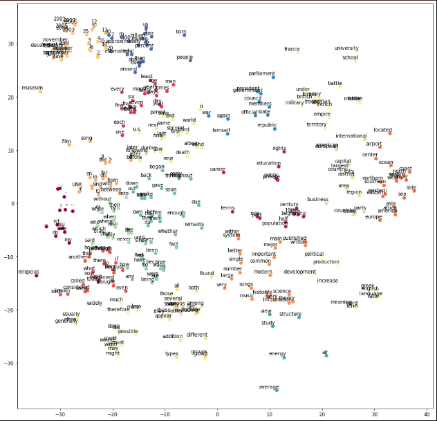
6.8 visual skip gram learning process
I just took a brief look at the visualization here. Because the core is still in the learning process, I just pasted the code and the comments I wrote at that time.
6.8.1 find only clustered words instead of sparsely distributed words
def find_clustered_embeddings(embeddings,distance_threshold,sample_threshold):
    '''
    Find only the closely clustered embeddings.
    This gets rid of more sparsly distributed word embeddings and make the visualization clearer
    This is useful for t-SNE visualization

    distance_threshold: maximum distance between two points to qualify as neighbors
    sample_threshold: number of neighbors required to be considered a cluster
    '''

    # calculate cosine similarity
    cosine_sim = np.dot(embeddings,np.transpose(embeddings))
    norm = np.dot(np.sum(embeddings**2,axis=1).reshape(-1,1),np.sum(np.transpose(embeddings)**2,axis=0).reshape(1,-1))
    assert cosine_sim.shape == norm.shape
    cosine_sim /= norm  # Obtain cosine similarity

    # make all the diagonal entries zero otherwise this will be picked as highest
    # Here, the diagonal element is the dot product of the vector of the word i and itself
    # That is to say, the similarity between yourself and yourself is not considered (because the similarity between yourself and yourself is the highest)
    np.fill_diagonal(cosine_sim, -1.0)  # Put cosine_ The diagonal element of SIM becomes - 1

    argmax_cos_sim = np.argmax(cosine_sim, axis=1)
    mod_cos_sim = cosine_sim
    # find the maximums in a loop to count if there are more than n items above threshold
    # Set the maximum value of each row to - 1
    for _ in range(sample_threshold-1):
        argmax_cos_sim = np.argmax(cosine_sim, axis=1)  # Select a maximum value for each iteration
        mod_cos_sim[np.arange(mod_cos_sim.shape[0]),argmax_cos_sim] = -1  # Set the maximum value selected in this round of iteration to - 1

    max_cosine_sim = np.max(mod_cos_sim,axis=1)  # After the iteration, select the largest element in the current matrix

    return np.where(max_cosine_sim>distance_threshold)[0]
6.8.2 t-SNE visualization with sklearn computing word embedding
num_points = 1000 # we will use a large sample space to build the T-SNE manifold and then prune it using cosine similarity

tsne = TSNE(perplexity=30, n_components=2, init='pca', n_iter=5000)

print('Fitting embeddings to T-SNE. This can take some time ...')
# get the T-SNE manifold
selected_embeddings = skip_gram_final_embeddings[:num_points, :]  # Extract the first 1000 embedded vectors
two_d_embeddings = tsne.fit_transform(selected_embeddings)

print('Pruning the T-SNE embeddings')
# prune the embeddings by getting ones only more than n-many sample above the similarity threshold
# this unclutters the visualization
selected_ids = find_clustered_embeddings(selected_embeddings,.25,10)  # Get the id of the clustered word
two_d_embeddings = two_d_embeddings[selected_ids,:]

print('Out of ',num_points,' samples, ', selected_ids.shape[0],' samples were selected by pruning')
6.8.3 use matplotlib to draw the diagram of t-SNE
def plot(embeddings, labels):

    n_clusters = 20 # number of clusters
    # automatically build a discrete set of colors, each for cluster
    label_colors = [pylab.cm.Spectral(float(i) /n_clusters) for i in range(n_clusters)]

    assert embeddings.shape[0] >= len(labels), 'More labels than embeddings'

    # Define K-Means
    kmeans = KMeans(n_clusters=n_clusters, init='k-means++', random_state=0).fit(embeddings)
    kmeans_labels = kmeans.labels_

    pylab.figure(figsize=(15,15))  # in inches

    # plot all the embeddings and their corresponding words
    for i, (label,klabel) in enumerate(zip(labels,kmeans_labels)):
        x, y = embeddings[i,:]
        pylab.scatter(x, y, c=label_colors[klabel])

        pylab.annotate(label, xy=(x, y), xytext=(5, 2), textcoords='offset points',
                       ha='right', va='bottom',fontsize=10)

    # use for saving the figure if needed
    #pylab.savefig('word_embeddings.png')
    pylab.show()

words = [reverse_dictionary[i] for i in selected_ids]
plot(two_d_embeddings, words)
The generated diagram is as follows:
7 CBOW
7.1 change the data generation process
Because the network structure of CBOW and skip gram is different, the data generation process needs to be changed. The network structure of CBOW is as follows:
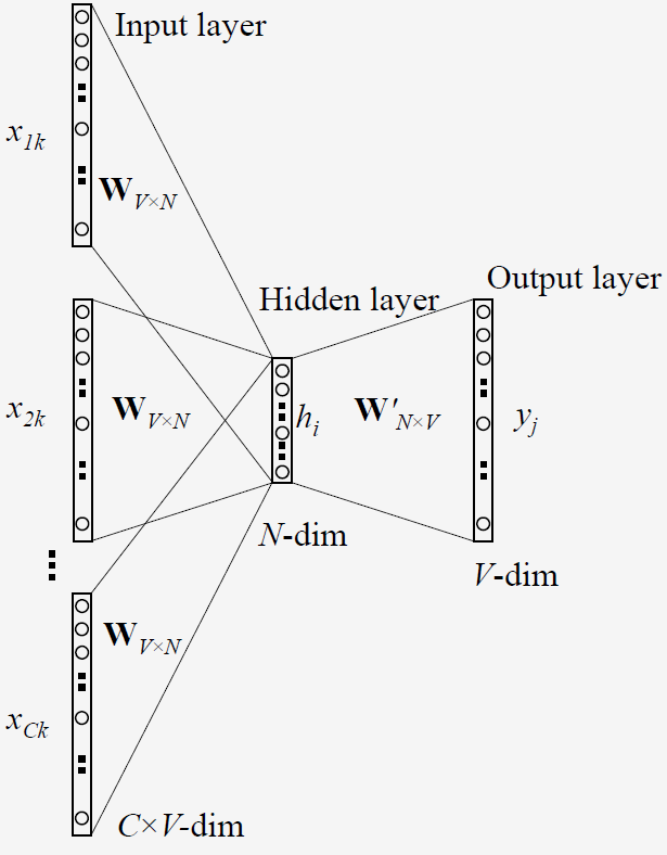
Since CBOW has multiple inputs, the size of the input vector varies from
b
a
t
c
h
_
s
i
z
e
×
1
{\rm batch\_size \times 1}
batch_size × 1 becomes
b
a
t
c
h
_
s
i
z
e
×
(
c
o
n
t
e
x
t
_
w
i
n
d
o
w
∗
2
)
{\rm batch\_size} \times ({\rm context\_window} * 2)
batch_size×(context_window∗2).
data_index = 0

def generate_batch_cbow(batch_size, window_size):
    # window_size is the amount of words we're looking at from each side of a given word
    # creates a single batch
    # The input is the context of the word i, and the one-sided context has window_size words

    # data_index is updated by 1 everytime we read a set of data point
    global data_index

    # span defines the total window size, where
    # data we consider at an instance looks as follows.
    # [ skip_window target skip_window ]
    # e.g if skip_window = 2 then span = 5
    # Left and right contextual words + target words
    span = 2 * window_size + 1 # [ skip_window target skip_window ]

    # two numpy arras to hold target words (batch)
    # and context words (labels)
    # Note that batch has span-1=2*window_size columns
    # batch: the context word of the target word
    # labels: target word
    batch = np.ndarray(shape=(batch_size,span-1), dtype=np.int32)
    labels = np.ndarray(shape=(batch_size, 1), dtype=np.int32)

    # The buffer holds the data contained within the span
    buffer = collections.deque(maxlen=span)

    # Fill the buffer and update the data_index
    for _ in range(span):
        buffer.append(data[data_index])
        data_index = (data_index + 1) % len(data)

    # Here we do the batch reading
    # We iterate through each batch index
    # For each batch index, we iterate through span elements
    # to fill in the columns of batch array
    # i: Record the index of the target word
    for i in range(batch_size):
        target = window_size  # target label at the center of the buffer
        target_to_avoid = [ window_size ] # we only need to know the words around a given word, not the word itself

        # add selected target to avoid_list for next time
        col_idx = 0  # Record the index of context words in batch
        # j: Record the index of context words in buffer
        for j in range(span):
            # ignore the target word when creating the batch
            if j==span//2:
                continue
            batch[i,col_idx] = buffer[j]
            col_idx += 1
        labels[i, 0] = buffer[target]

        # Everytime we read a data point,
        # we need to move the span by 1
        # to create a fresh new span
        # Move sliding window
        buffer.append(data[data_index])
        data_index = (data_index + 1) % len(data)

    return batch, labels

print('data:', [reverse_dictionary[di] for di in data[:8]])

for window_size in [1,2]:
    data_index = 0
    batch, labels = generate_batch_cbow(batch_size=8, window_size=window_size)
    print('\nwith window_size = %d:' % (window_size))
    print('    batch:', [[reverse_dictionary[bii] for bii in bi] for bi in batch])
    print('    labels:', [reverse_dictionary[li] for li in labels.reshape(8)])
Generate here and in 5_ batch_ skip_ Gram () is similar, except that batch and labels are different.
for i in range(batch_size):
    target = window_size  # target label at the center of the buffer
    target_to_avoid = [ window_size ] # we only need to know the words around a given word, not the word itself

    # add selected target to avoid_list for next time
    col_idx = 0  # Record the index of context words in batch
    # j: Record the index of context words in buffer
    for j in range(span):
        # ignore the target word when creating the batch
        if j==span//2:
            continue
        batch[i,col_idx] = buffer[j]
        col_idx += 1
    labels[i, 0] = buffer[target]

    # Everytime we read a data point,
    # we need to move the span by 1
    # to create a fresh new span
    # Move sliding window
    buffer.append(data[data_index])
    data_index = (data_index + 1) % len(data)
span // 2 is used here to skip the target word. Because CBOW predicts the target word according to the context, the target word becomes labels, and the input word becomes the context of the target word. Because the target word and its context are recorded in the buffer, the subscript of the target word needs to be skipped during the loop. In each cycle, labels records the predicted words and batch records the contextual words.
The output is as follows:
data: ['propaganda', 'is', 'a', 'concerted', 'set', 'of', 'messages', 'aimed']

with window_size = 1:
    batch: [['propaganda', 'a'], ['is', 'concerted'], ['a', 'set'], ['concerted', 'of'], ['set', 'messages'], ['of', 'aimed'], ['messages', 'at'], ['aimed', 'influencing']]
    labels: ['is', 'a', 'concerted', 'set', 'of', 'messages', 'aimed', 'at']

with window_size = 2:
    batch: [['propaganda', 'is', 'concerted', 'set'], ['is', 'a', 'set', 'of'], ['a', 'concerted', 'of', 'messages'], ['concerted', 'set', 'messages', 'aimed'], ['set', 'of', 'aimed', 'at'], ['of', 'messages', 'at', 'influencing'], ['messages', 'aimed', 'influencing', 'the'], ['aimed', 'at', 'the', 'opinions']]
    labels: ['a', 'concerted', 'set', 'of', 'messages', 'aimed', 'at', 'influencing']
7.2 defining super parameters
batch_size = 128 # Data points in a single batch
embedding_size = 128 # Dimension of the embedding vector.
# How many words to consider left and right.
# Skip gram by design does not require to have all the context words in a given step
# However, for CBOW that's a requirement, so we limit the window size
window_size = 2

# We pick a random validation set to sample nearest neighbors
valid_size = 16 # Random set of words to evaluate similarity on.
# We sample valid datapoints randomly from a large window without always being deterministic
valid_window = 50

# When selecting valid examples, we select some of the most frequent words as well as
# some moderately rare words as well
valid_examples = np.array(random.sample(range(valid_window), valid_size))
valid_examples = np.append(valid_examples,random.sample(range(1000, 1000+valid_window), valid_size),axis=0)

num_sampled = 32 # Number of negative examples to sample.
batch_size: number of samples in a batch
embedding_size: the size of the embedded vector (hidden layer)
window_size: context size
7.3 defining inputs and outputs
tf.reset_default_graph()

# Training input data (target word IDs). Note that it has 2*window_size columns
train_dataset = tf.placeholder(tf.int32, shape=[batch_size,2*window_size])
# Training input label data (context word IDs)
train_labels = tf.placeholder(tf.int32, shape=[batch_size, 1])
# Validation input data, we don't need a placeholder
# as we have already defined the IDs of the words selected
# as validation data
valid_dataset = tf.constant(valid_examples, dtype=tf.int32)
train_dataset: the training dataset entered in each batch, with the size of
128
×
4
128 \times 4
one hundred and twenty-eight × 4, (each input has 4 contexts)
train_labels: entered label, size
128
×
1
128 \times 1
one hundred and twenty-eight × 1, (there is only one output word for every four input contexts)
valid_dataset: validation set
7.4 defining model parameters and other variables
embeddings: weight matrix from input layer to hidden layer W W W, V × N V \times N V × N. Evenly distributed [ − 1 , 1 ] [-1, 1] [−1,1].
softmax_weights: hidden layer to output layer weights W ′ W' W′, V × N V \times N V × N. Truncated normal distribution, mean 0, standard deviation 0.5 128 \frac{0.5}{\sqrt{128}} 128 0.5
softmax_ Bias: bias of output layer b b b, V V 5. Evenly distributed [ 0 , 0.01 ] [0, 0.01] [0,0.01]
# Variables.

# Embedding layer, contains the word embeddings
embeddings = tf.Variable(tf.random_uniform([vocabulary_size, embedding_size], -1.0, 1.0,dtype=tf.float32))

# Softmax Weights and Biases
softmax_weights = tf.Variable(tf.truncated_normal([vocabulary_size, embedding_size],
                              stddev=0.5 / math.sqrt(embedding_size),dtype=tf.float32))
softmax_biases = tf.Variable(tf.random_uniform([vocabulary_size],0.0,0.01))
7.5 definition model calculation
# Model.
# Look up embeddings for a batch of inputs.
# Here we do embedding lookups for each column in the input placeholder
# and then average them to produce an embedding_size word vector
stacked_embedings = None  # The context vector of each target word constitutes a matrix
print('Defining %d embedding lookups representing each word in the context'%(2*window_size))
for i in range(2*window_size):
    embedding_i = tf.nn.embedding_lookup(embeddings, train_dataset[:,i])  # Take out the train_ embedding vector of words in column i of dataset
    x_size,y_size = embedding_i.get_shape().as_list()
    if stacked_embedings is None:
        stacked_embedings = tf.reshape(embedding_i,[x_size,y_size,1])
    else:
        stacked_embedings = tf.concat(axis=2,values=[stacked_embedings,tf.reshape(embedding_i,[x_size,y_size,1])])

assert stacked_embedings.get_shape().as_list()[2]==2*window_size
print("Stacked embedding size: %s"%stacked_embedings.get_shape().as_list())
mean_embeddings =  tf.reduce_mean(stacked_embedings,2,keepdims=False)  # Sum and average the input vectors
print("Reduced mean embedding size: %s"%mean_embeddings.get_shape().as_list())

# Compute the softmax loss, using a sample of the negative labels each time.
# inputs are embeddings of the train words
# with this loss we optimize weights, biases, embeddings
loss = tf.reduce_mean(
    tf.nn.sampled_softmax_loss(weights=softmax_weights, biases=softmax_biases, inputs=mean_embeddings,
                               labels=train_labels, num_sampled=num_sampled, num_classes=vocabulary_size))
The output is as follows:
Defining 4 embedding lookups representing each word in the context
Stacked embedding size: [128, 128, 4]
Reduced mean embedding size: [128, 128]
This step is mainly to find the input vector. Because CBOW is to input multiple contexts, these contexts need to be averaged before they can be submitted to the hidden layer. The function of this for loop is to splice the input vectors, and then use TF reduce_ Mean() averages.
The loss function is the same as that defined by skip gram model, so I won't repeat it.
7.6 model parameter optimizer
Here, Adagrad is also used as the optimizer.
# Optimizer.
optimizer = tf.train.AdagradOptimizer(1.0).minimize(loss)
7.7 calculating word similarity
# Compute the similarity between minibatch examples and all embeddings.
# We use the cosine distance:
norm = tf.sqrt(tf.reduce_sum(tf.square(embeddings), 1, keepdims=True))
normalized_embeddings = embeddings / norm
valid_embeddings = tf.nn.embedding_lookup(normalized_embeddings, valid_dataset)
similarity = tf.matmul(valid_embeddings, tf.transpose(normalized_embeddings))
This is as like as two peas before, and not much more.
7.8 running CBOW model
num_steps = 100001
cbow_losses = []

# ConfigProto is a way of providing various configuration settings
# required to execute the graph
with tf.Session(config=tf.ConfigProto(allow_soft_placement=True)) as session:

    # Initialize the variables in the graph
    tf.global_variables_initializer().run()
    print('Initialized')

    average_loss = 0

    # Train the Word2vec model for num_step iterations
    for step in range(num_steps):

        # Generate a single batch of data
        batch_data, batch_labels = generate_batch_cbow(batch_size, window_size)

        # Populate the feed_dict and run the optimizer (minimize loss)
        # and compute the loss
        feed_dict = {train_dataset : batch_data, train_labels : batch_labels}
        _, l = session.run([optimizer, loss], feed_dict=feed_dict)

        # Update the average loss variable
        average_loss += l

        if (step+1) % 2000 == 0:
            if step > 0:
                average_loss = average_loss / 2000
                # The average loss is an estimate of the loss over the last 2000 batches.
            cbow_losses.append(average_loss)
            print('Average loss at step %d: %f' % (step+1, average_loss))
            average_loss = 0

        # Evaluating validation set word similarities
        if (step+1) % 10000 == 0:
            sim = similarity.eval()
            # Here we compute the top_k closest words for a given validation word
            # in terms of the cosine distance
            # We do this for all the words in the validation set
            # Note: This is an expensive step
            for i in range(valid_size):
                valid_word = reverse_dictionary[valid_examples[i]]
                top_k = 8 # number of nearest neighbors
                nearest = (-sim[i, :]).argsort()[1:top_k+1]
                log = 'Nearest to %s:' % valid_word
                for k in range(top_k):
                    close_word = reverse_dictionary[nearest[k]]
                    log = '%s %s,' % (log, close_word)
                print(log)
    cbow_final_embeddings = normalized_embeddings.eval()


np.save('cbow_embeddings',cbow_final_embeddings)

with open('cbow_losses.csv', 'wt') as f:
    writer = csv.writer(f, delimiter=',')
    writer.writerow(cbow_losses)
The only difference between this and skip gram is the generated batch_data and batch_labels are different, so the parameters passed in loss are different.
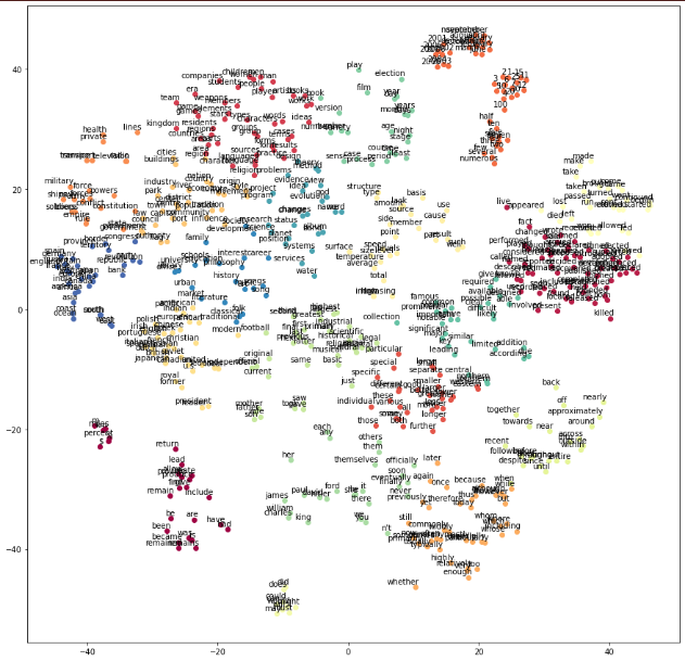
7.9 visual CBOW learning process
7.9.1 using sklearn computing words to embed t-SNE visualization
num_points = 1000 # we will use a large sample space to build the T-SNE manifold and then prune it using cosine similarity

tsne = TSNE(perplexity=30, n_components=2, init='pca', n_iter=5000)

print('Fitting embeddings to T-SNE. This can take some time ...')
# get the T-SNE manifold
selected_embeddings = cbow_final_embeddings[:num_points, :]  # Extract the first 1000 embedded vectors
two_d_embeddings = tsne.fit_transform(selected_embeddings)

print('Pruning the T-SNE embeddings')
# prune the embeddings by getting ones only more than n-many sample above the similarity threshold
# this unclutters the visualization
selected_ids = find_clustered_embeddings(selected_embeddings,.25,10)  # Get the id of the clustered word
two_d_embeddings = two_d_embeddings[selected_ids,:]

print('Out of ',num_points,' samples, ', selected_ids.shape[0],' samples were selected by pruning')
7.9.2 using matplotlib to draw t-SNE
def plot(embeddings, labels):

    n_clusters = 20 # number of clusters
    # automatically build a discrete set of colors, each for cluster
    label_colors = [pylab.cm.Spectral(float(i) /n_clusters) for i in range(n_clusters)]

    assert embeddings.shape[0] >= len(labels), 'More labels than embeddings'

    # Define K-Means
    kmeans = KMeans(n_clusters=n_clusters, init='k-means++', random_state=0).fit(embeddings)
    kmeans_labels = kmeans.labels_

    pylab.figure(figsize=(15,15))  # in inches

    # plot all the embeddings and their corresponding words
    for i, (label,klabel) in enumerate(zip(labels,kmeans_labels)):
        x, y = embeddings[i,:]
        pylab.scatter(x, y, c=label_colors[klabel])

        pylab.annotate(label, xy=(x, y), xytext=(5, 2), textcoords='offset points',
                       ha='right', va='bottom',fontsize=10)

    # use for saving the figure if needed
    #pylab.savefig('word_embeddings.png')
    pylab.show()

words = [reverse_dictionary[i] for i in selected_ids]
plot(two_d_embeddings, words)
8 reference
[1] Thushan Ganegedara. Natural language processing with tensorflow [M] Beijing: China Machine Press, 2019: 42-46
[2] Wild pointer Xiao Li Detailed derivation of Word2Vec principle and formula [EB / OL] (2021-04-28)[2021-06-18]. https://blog.csdn.net/qq_35357274/article/details/116240180
[3] Wild pointer Xiao Li Word2Vec's Hierarchical Softmax and negative sampling [EB / OL] (2021-05-03)[2021-06-18]. https://blog.csdn.net/qq_35357274/article/details/116381205
[4] 101 Huanhuan fish python——random. Usage of sample() [EB / OL] (2019-08-12)[2021-06-18]. https://www.cnblogs.com/fish-101/p/11339909.html
[5] TaoTao Yu. embedding_ Study notes for lookup [EB / OL] (2019-08-04)[2021-06-18]. https://blog.csdn.net/hit0803107/article/details/98377030
[6] Ah often talks nonsense Use of deque in collections [EB / OL] (2018-06-21)[2021-06-18]. https://blog.csdn.net/u010339879/article/details/80767293