Dropout Solves overfitting

 

overfitting is also known as over-learning and over-fitting. He is a common problem in machine learning.

 

 

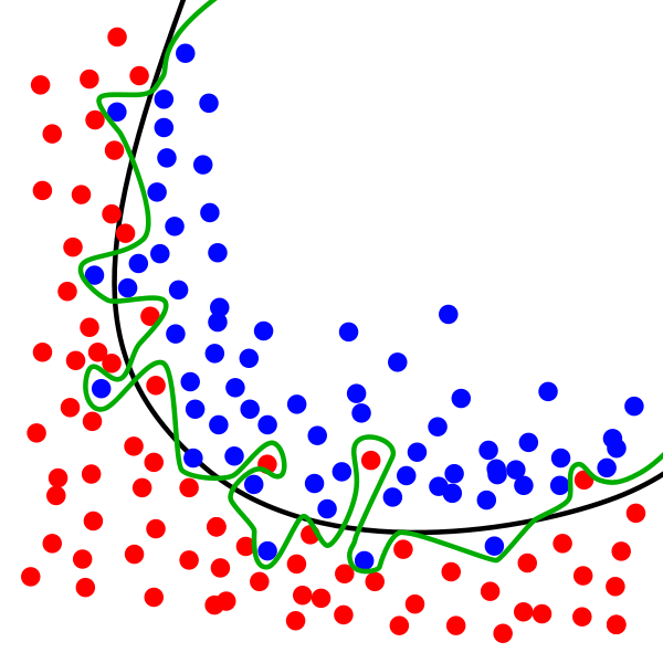
The black curve is the normal model, and the green curve is the overfitting model. Although the green curve accurately distinguishes all the training data, it does not describe the overall characteristics of the data and has poor adaptability to the new test data.

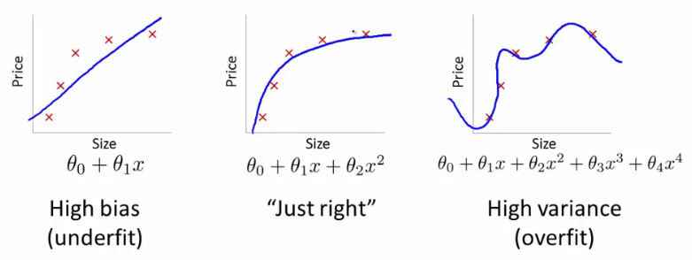
Take Regression for example.

 

The third curve has the problem of overfitting. Although it passes through all training points, it can not reflect the trend of data very well, and its prediction ability is seriously inadequate. tensorflow provides a powerful drop out method to end overfitting problems.

 

Establishment of Dropout Layer

This content needs to install data adapted to sklearn database. Students who do not install sklearn can refer to the following

import tensorflow as tf
from sklearn.datasets import load_digits
from sklearn.model_selection import train_test_split
from sklearn.preprocessing import  LabelBinarizer

keep_prob = tf.placeholder(tf.float32)
...
...
Wx_plus_b = tf.nn.dropout(Wx_plus_b, keep_prob)

Here keep_prob is the retention probability, that is, the proportion of the results we want to retain. As a placeholder, it is passed in when run. When keep_prob=1, it is equivalent to 100% retention, that is, drop does not work.

 

The following data are prepared:

digits = load_digits()
X = digits.data
y = digits.target
y = LabelBinarizer().fit_transform(y)
X_train, X_test, y_train, y_test = train_test_split(X, y, test_size=.3)

X_train is the training data and X_test is the test data. Then add the hidden layer and output layer

 

# add output layer
l1 = add_layer(xs, 64, 50, 'l1', activation_function=tf.nn.tanh)
prediction = add_layer(l1, 50, 10, 'l2', activation_function=tf.nn.softmax)

The activation function of adding layer is tanh (actually I don't know why, I don't bother to write tanh function in class, other functions will report none error, no matter what)

 

train

sess.run(train_step, feed_dict={xs: X_train, ys: y_train, keep_prob: 0.5})
#sess.run(train_step, feed_dict={xs: X_train, ys: y_train, keep_prob: 1})

Preservation probability refers to how much is retained. Let's try 0.5-1.0 to observe the visualization results generated by tensorboard.

 

Visualization results

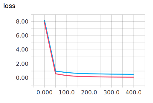
When keep_prob=1, the problem of overfitting will be exposed. When keep_prob=0.5, Dropout will play a role.

When keep_prob=1, the adaptability of the model to training data is better than that of test data, and there exists overfitting. The red line is the error of train and the blue line is the error of test.

 

When keep_prob=0.5

You can clearly see the changes in loss

 

The complete code and some comments are as follows

import tensorflow as tf
from sklearn.datasets import load_digits
from sklearn.model_selection import train_test_split
from sklearn.preprocessing import  LabelBinarizer

#Load data
digits = load_digits()
X = digits.data
y = digits.target
#preprocessing.LabelBinarizer It's a very useful tool.
# For example, you can yes and no Convert to 0 and 1
# Or incident and normal Convert to 0 and 1
y = LabelBinarizer().fit_transform(y)
X_train,X_test,y_train,y_test = train_test_split(X,y,test_size=.3)

def add_layer(inputs,in_size,out_size,layer_name,activation_function=None,):
    Weights = tf.Variable(tf.random_normal([in_size,out_size]))
    biases = tf.Variable(tf.zeros([1,out_size])+ 0.1)
    Wx_plus_b = tf.matmul(inputs,Weights)+biases
    #here to drop
    Wx_plus_b = tf.nn.dropout(Wx_plus_b, keep_prob)
    if activation_function is None:
        outputs = Wx_plus_b
    else:
        outputs = activation_function(Wx_plus_b,)
    tf.summary.histogram(layer_name + 'outputs',outputs)
    return outputs

#define placeholder for inputs to network
keep_prob = tf.placeholder(tf.float32)#Retention probability is the proportion of the results we need to retain
xs = tf.placeholder(tf.float32,[None,64])#8*8
ys = tf.placeholder(tf.float32,[None,10])

#add output layer
l1 = add_layer(xs,64,50,'l1',activation_function=tf.nn.tanh)
prediction = add_layer(l1,50,10,'l2',activation_function=tf.nn.softmax)

#the loss between prediction and real data
#loss
cross_entropy = tf.reduce_mean(-tf.reduce_sum(ys*tf.log(prediction),reduction_indices=[1]))

tf.summary.scalar('loss',cross_entropy)
train_step = tf.train.GradientDescentOptimizer(0.5).minimize(cross_entropy)

sess = tf.Session()
merged = tf.summary.merge_all()

#summary writer goes in here
train_writer = tf.summary.FileWriter("logs/train",sess.graph)
test_writer = tf.summary.FileWriter("logs/test",sess.graph)

init = tf.global_variables_initializer() #Variable initialization

sess.run(init)

for i in range(500):
    #here to determine the keeping probability
    sess.run(train_step,feed_dict={xs:X_train,ys:y_train,keep_prob:0.5})
    if i %50 ==0:
        #record loss
        train_result = sess.run(merged,feed_dict={xs:X_train,ys:y_train,keep_prob:1})
        test_result = sess.run(merged,feed_dict={xs:X_test,ys:y_test,keep_prob:1})
        train_writer.add_summary(test_result,i)
        test_writer.add_summary(test_result,i)