overview

For those detectors running on GPU platform, their backbone network may be VGG, ResNet, ResNeXt or DenseNet.

For those detectors running on the CPU platform, their detectors may be SqueezeNet, MobileNet and shufflenet.

The most representative two-stage target detector R-CNN series include fast R-CNN, fast R-CNN, R-FCN [9], Libra R-CNN. The two-stage target detector can also be made an anchor free target detector, such as RepPoints. As for the one-stage target detector, the most representative networks include YOLO, SSD and RetinaNet.

The anchor free target detector in the first stage is developing continuously, including CenterNet, CornerNet, FCOS, etc. In recent years, the target detector usually adds some layers between the head and the backbone network. These layers are used to collect feature maps at different stages. The networks with this mechanism include Feature Pyramid Network (FPN), Path Aggregation Network (PAN), BiFPN and NAS-FPN.

In addition to the above models, some researchers focus on the research backbone network (DetNet, DetNAS), while others are committed to building a new model for target detection (SpineNet, HitDetector).

Generally speaking, the general target detector consists of the following parts:

• Input: Image, Patches, Image Pyramid
• Backbones: VGG16, ResNet-50,SpineNet，EffificientNet-B0/B7, CSPResNeXt50， CSPDarknet53
• Neck:
• Additional blocks: SPP,ASPP,RFB，SAM
• Path-aggregation blocks: FPN，PAN，NAS-FPN，Fully-connected FPN，BiFPN，ASFF，SFAM
• Heads:
• Dense Prediction(one-stage):
  • RPN，SSD，YOLO，RetinaNet(anchor based)
  • CornerNet，CenterNet，MatrixNet，FCOS(anchor free)
• Sparse Prediction(two-stage):
• • Faster R-CNN，R-FCN，Mask R-CNN(anchor based)
  • RepPoints(anchor free)
    ​

1, What is YOLO

YOLO is the abbreviation of "You Only Look Once". Although it is not the most accurate algorithm, the compromise between accuracy and speed is also quite good. YOLOv3 draws lessons from YOLOv1 and YOLOv2. Although there are not many innovations, it improves the detection accuracy while maintaining the speed advantage of YOLO family, especially for small objects. YOLOv3 algorithm uses a single neural network to act on the image, divides the image into multiple regions, and predicts the boundary box and the probability of each region.

2, YOLOv3 network

1. Network structure

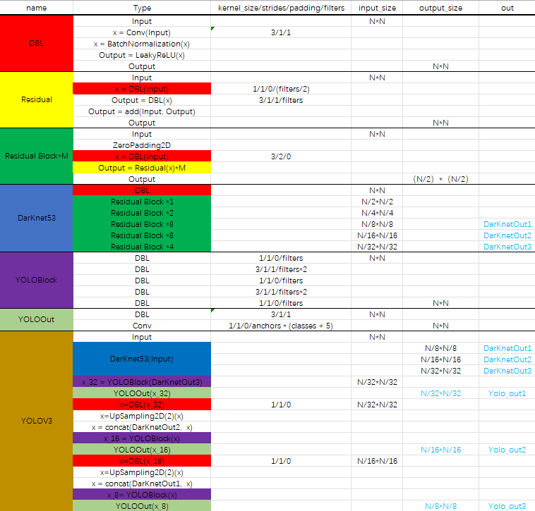
The feature extraction part (backbone) of yolov3 network adopts Darkenet53. Yolov3 uses the 52 layers in front of darknet-53 (without full connection layer). Yolov3 network is a full convolution network, which uses a lot of residual layer hopping connection. In order to reduce the negative effect of gradient caused by POOLing, the author directly abandons POOLing and uses conv's stripe to realize downsampling. In this network structure, the convolution with step size of 2 is used for downsampling.

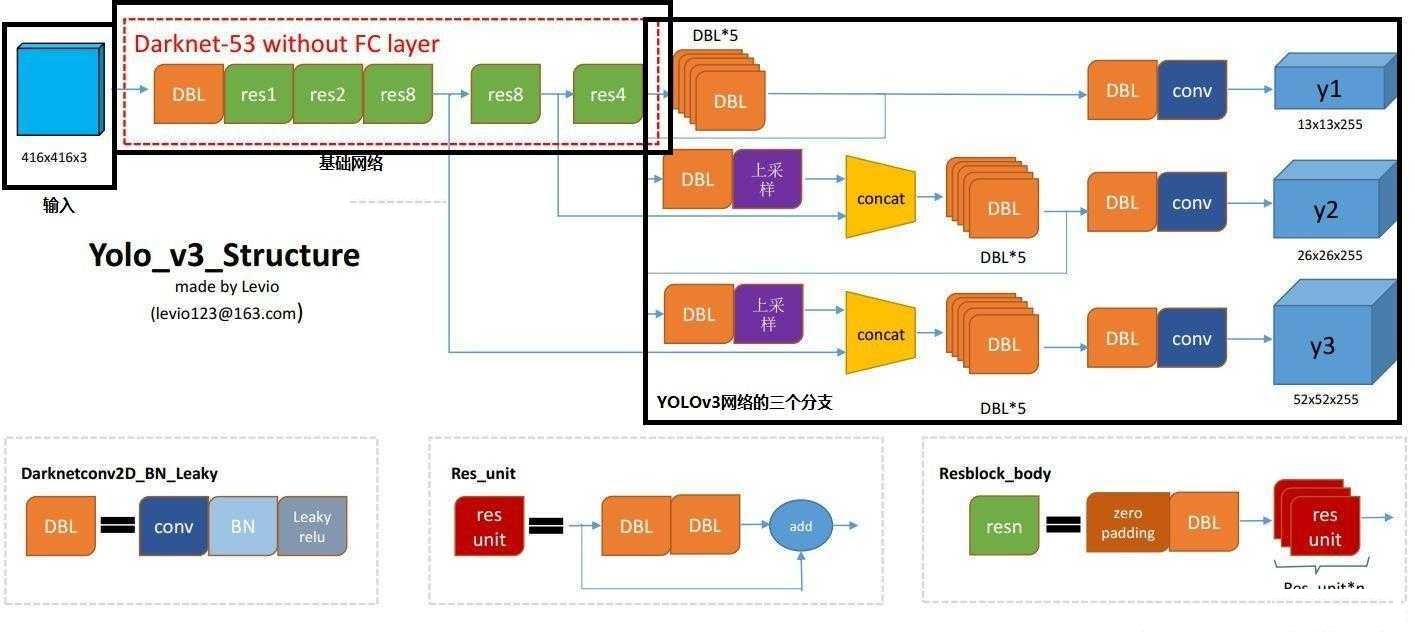
DBL: darknetconv2d in code_ BN_ Leaky, it's Yolo_ Basic components of v3. Convolution + BN+Leaky relu.

Residual block * m: m stands for number, indicating how many residuals are contained in this ResidualBlock

concat: tensor splicing. Splice the upper samples of the middle layer of darknet and a layer behind it. The operation of splicing is different from that of add in the residual layer. Splicing will expand the dimension of tensor, while add is only a direct addition and will not change the dimension of tensor.

Network structure analysis:

1. In Yolov3, there is only convolution layer, and the size of the output characteristic graph is controlled by adjusting the convolution step size. Therefore, there are no special restrictions on the size of the input picture.

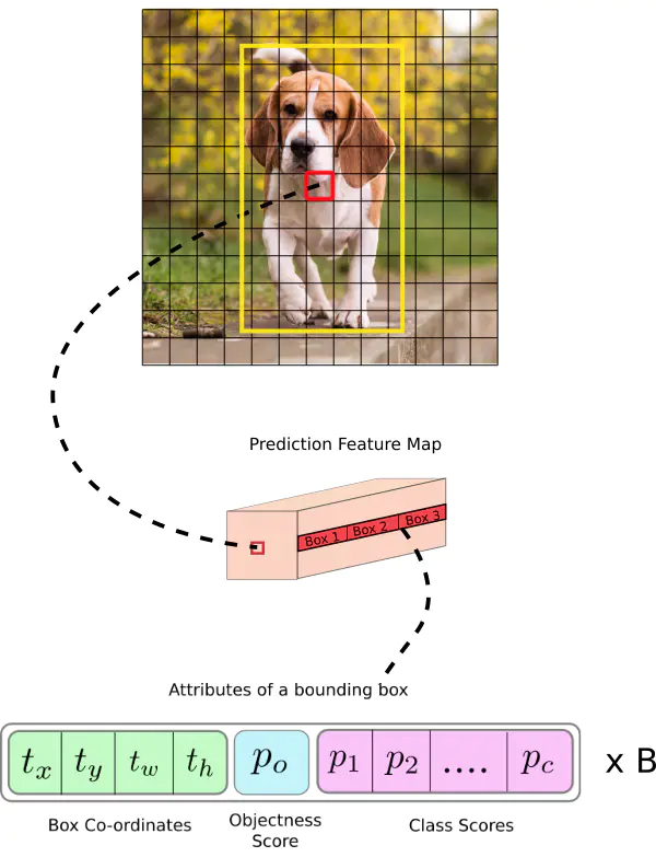
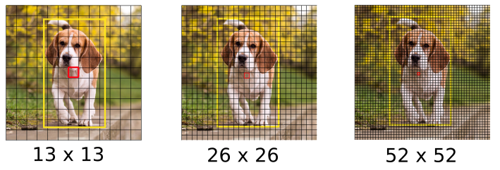
2. Yolov3 draws lessons from the idea of pyramid feature map. Small-scale feature map is used to detect large-scale objects, while large-scale feature map detects small-scale objects. The output dimension of the feature graph is n × N × [3 × (4 + 1 + 80)]， N × N is the number of output feature grid points. There are 3 Anchor boxes in total, and each box has a 4-dimensional prediction box value , 1-dimensional prediction frame confidence, number of 80 dimensional object categories. Therefore, the output dimension of the first layer feature graph is 13 × thirteen × 255.

3. yolov3 outputs a total of three feature maps. The first feature map is sampled 32 times, the second feature map is sampled 16 times, and the third feature map is sampled 8 times. The feature map generated by the input image through Darknet-53 (no full connection layer) and Yoloblock is regarded as dual-purpose. The first is to generate feature map I after 33 convolution layers and 11 convolution, and the second is to generate feature map 1 after 1 convolution × 1. The convolution layer and sampling layer are spliced with the output results of the middle layer of Darnet-53 network to produce characteristic figure 2. After the same cycle, characteristic figure 3 is generated.

4. The difference between concat operation and addition operation: the addition operation comes from ResNet idea, which adds the corresponding dimensions of the input characteristic diagram and the output characteristic diagram, that is, y = f(x) + x; The concat operation originates from the design idea of DenseNet network, which directly splices the feature map according to the channel dimension, such as 13 × thirteen × Characteristic diagram of 16 and 13 × thirteen × The feature map of 16 is spliced to generate 13 × thirteen × 32.

5. Upsample: it is used to generate large-scale images from small-scale feature images through interpolation and other methods. For example, using the nearest neighbor interpolation algorithm, 13 × The image of 13 is transformed into 26 × 26. The upper sampling layer does not change the number of channels of the characteristic graph.

Yolo's entire network absorbs the essence of Resnet, densinet and FPN, which can be said to integrate all the most effective techniques in the current industry of target detection.

2. Interpretation of network output (forward process)

2.1 size of output characteristic drawing

According to different input sizes, output characteristic diagrams of different sizes will be obtained, and the output characteristic diagram is 13 × thirteen × 255,26 × twenty-six × 255,52 × fifty-two × 255. In the design of Yolov3, each grid of each feature graph is configured with three different a priori frames, so the last three feature graphs, here for the time being, reshape is 13 × thirteen × three × 85,26 × twenty-six × three × 85,52 × fifty-two × three × 85, which is easier to understand and easier to operate after reshape is formed in the code. The three characteristic graphs are the detection results output by the whole Yolo. The position of the detection frame (4D), the detection confidence (1D) and the category (80D) are all in them, and the total is exactly 85D. The last dimension 85 of the feature map represents this information, while the other dimensions n of the feature map × N × 3，N × N represents the reference position information of the detection frame, and 3 is a priori frame of three different scales.

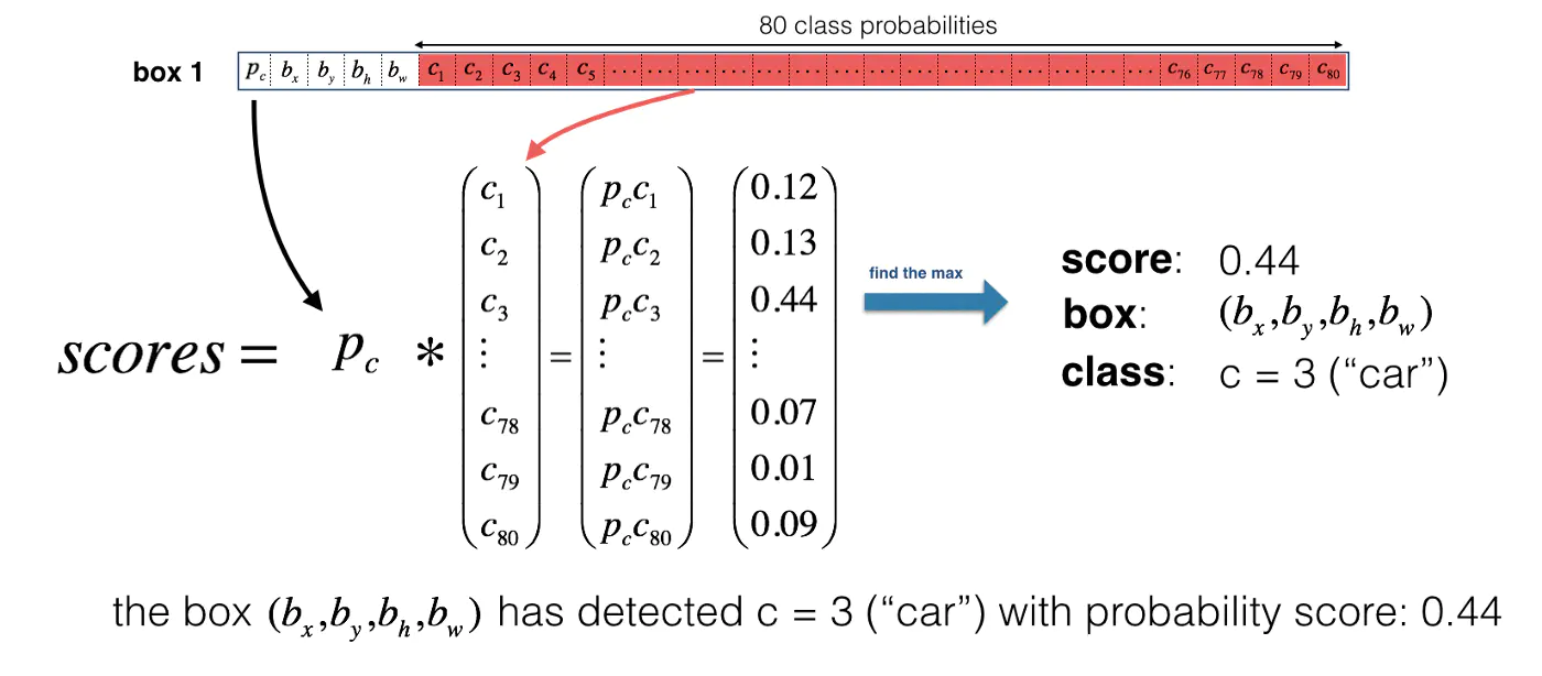
Now, for each anchor box of each cell, we calculate the following element level multiplication and get the probability that the anchor box contains an object class, as shown in the following figure:

2.2 anchor frame and prediction

• A priori frame

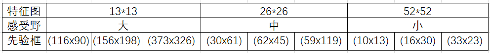
In Yolov1, the network directly regresses the width and height of the detection frame, so the effect is limited. Therefore, in Yolov2, it is changed to return the change value based on the a priori box, so that the learning difficulty of the network is reduced and the overall accuracy is improved. Yolov3 follows the technique of a priori box in Yolov2, and uses k-means to cluster the label boxes in the data set to obtain 9 boxes of the category center as a priori boxes. In the COCO dataset (all original pictures are resize d to 416) × 416), the nine boxes are (10) × 13)，(16 × 30)，(33 × 23)，(30 × 61)，(62 × 45)，(59 × 119)， (116 × 90)， (156 × 198)，(373 × 326), in the order of w × h.

Note: the a priori frame is only related to w and h of the detection frame, not x and y.

The network downsamples the input image to the first detection layer (), and the step is 32; Then, the feature map sampled twice on this layer and the same size as the above is stacked according to the channel, and the second detection layer is formed according to the step 16; Similarly, for the same up sampling process, the final detection layer step is 8. On each scale, each cell uses three anchor boxes to predict three boundary boxes, a total of nine anchor boxes. All anchor frames add up to a total of 10647

• Detection frame decoding

With a priori frame and output characteristic graph, the detection frames x, y, w, h can be decoded.

Here b_x, b_y, b_w, b_h is the center coordinate, width and height we predicted. t_x, t_y, t_w, t_h is the output of the network. c_x, c_y is the coordinate of the grid from the top to the left. p_w, p_h is the dimension of the anchor box

As shown in the figure below, it is the offset based on the grid coordinates in the upper left corner of the center point of the rectangular box. It is the activation function. In this paper, the author uses sigmoid. The center coordinate is predicted by sigmoid function, and the value is forcibly limited between 0 and 1. YOLO is not the absolute coordinate of the center of the prediction bounding box. It predicts the offset: relative to the upper left corner of the grid cell of the prediction object; Normalize the dimension through the characteristic map cell.
Consider the image of the dog above. If the prediction center coordinates are (0.4, 0.7), it means that the center is (because the coordinates in the upper left corner of the red box are (6, 6)). However, if the predicted coordinates are greater than 1, for example (1.2, 0.7), it means that the center is. Now the center is on the right side of the red box (7.2, 6.7), but we can only use the red box to be responsible for object prediction, so we add a sidmoid function to forcibly limit it between 0 and 1.

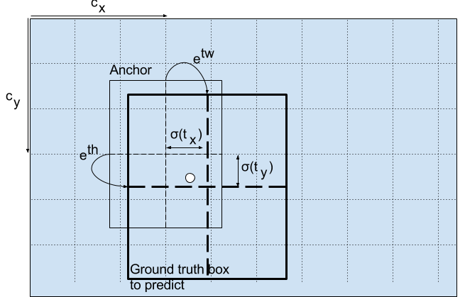Figure 3
For a specific example, suppose that for the second feature Figure 13 × thirteen × three × In the figure above, the second dimension in the [5] corresponds to a priori, and the second dimension in the [5] is a priori × 61)，(62 × 45)，(59 × 119)，prior_ If the index of box is 2, take the last 59119 as a priori w and a priori h. After such calculation, it is also necessary to multiply the sampling rate 13 of characteristic figure 2 to obtain the real detection frames x and y.

• Detection confidence decoding

Object detection confidence is very important in Yolo design, which is related to the detection accuracy and recall of the algorithm.

The confidence occupies a fixed bit in the output 85 dimension, which can be decoded by sigmoid function, and the numerical interval after decoding is in [0,1].

• Category decoding

The COCO dataset has 80 categories, so the number of categories accounts for 80 dimensions in the 85 dimensional output. Each dimension independently represents the confidence of a category. sigmoid activation function is used to replace softmax in Yolov2, eliminating the mutual exclusion between categories, which can make the network more flexible.

The three feature maps can decode a total of 13 × thirteen × 3 + 26 × twenty-six × 3 + 52 × fifty-two × 3 = 10647 boxes with corresponding category and confidence. The 10647 boxes are used differently in training and reasoning:

1. During training, all 10647 box es are sent to the labeling function for the next step of labeling and loss function calculation.
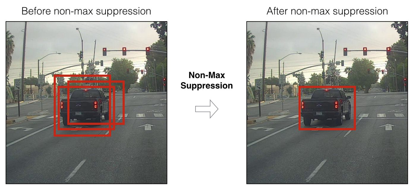
2. When reasoning, select a confidence threshold, filter out the low threshold box, and then output the prediction results of the whole network through nms (non maximum suppression).

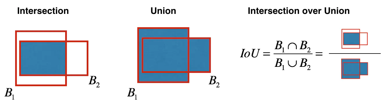
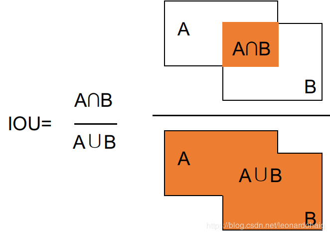
• The key to realize non maximum suppression is to select a box with the highest score; Calculate the coincidence degree between it and other frames, and remove the frames whose coincidence degree exceeds the IoU threshold; Go back to step 1 and iterate until there is no box lower than the currently selected box.

3. Training strategy and loss function (reverse process)

• Training strategy

The training strategies are summarized as follows:

1. The prediction box is divided into three cases: positive, negative and ignore.
2. Positive example: take any ground truth and calculate IOU with 4032 frames. The prediction frame with the largest IOU is a positive example. And a prediction box can only be assigned to one ground truth. For example, the first ground truth has matched a positive example detection box, then the next ground truth will find the detection box with the largest IOU as a positive example in the remaining 4031 detection boxes. The order of ground truth can be ignored. Positive examples generate confidence loss, detection frame loss and category loss. The prediction box is the corresponding ground truth box label; (reverse coding is required, and the corresponding TX, ty, TW, th of the category label is calculated by using the real x, y, w and h) the category is 1 and the rest is 0; The confidence label is 1.
3. Ignore the example: except for the positive example, if the IOU with any ground truth is greater than the threshold (0.5 is used in the paper), the example is ignored. Ignoring the sample does not produce any loss.
4. Negative example: except for the positive example (the largest detection frame of IOU after calculation with ground truth, but the IOU is less than the threshold, it is still a positive example), and the IOU with all ground truths is less than the threshold (0.5), it is a negative example. In the negative example, only the confidence level produces loss, and the confidence level label is 0.

• Loss function

The abstract expression of the loss function of Yolov3 in feature Figure 1 is as follows:

Yolov3 Loss is the sum of three characteristic graphs:

1. Is the weight constant, which controls the detection boxConfidence and The ratio between the confidence level Loss, usually the number of negative cases is more than dozens of times that of positive cases, and the detection effect can be controlled by weight hyperparameters.
2. If it is a positive example, it will output 1, otherwise it will be 0;If it is a negative example, it outputs 1, otherwise it is 0; Ignore the samples and output 0.
3. x. y, w and h use MSE as the loss function, or smooth L1 loss (from fast r-cnn) as the loss function. Smooth L1 can make the training smoother. Because the confidence and category labels are 0,1, the cross entropy is used as the loss function.

• Explanation of training strategy:

1. Why doesn't the ground truth allocate the corresponding prediction box according to the center point?

(1) In the training strategy of Yolov3, each cell is no longer responsible for the ground truth in the cell like Yolov1. The reason is that Yolov3 generates three feature maps in total. The centers of the cells on the three feature maps coincide. During training, the third box of characteristic figure 1 may be the most consistent, but during reasoning, the confidence of the first box of characteristic figure 2 is the highest. Therefore, Yolov3 training does not strictly allocate the specified cells according to the ground truth center point, but looks for the prediction frame with the largest IOU according to the prediction value as a positive example.

(2) First, the ground truth first determines the closest a priori frame from the nine a priori frames, so as to determine the number of feature maps and box positions to which the ground truth belongs, and then further allocate them according to the center point. Second, all 4032 output frames directly calculate the IOU with the ground truth, and allocate the ground truth to the cell with the highest IOU. The IOU value of the second calculation method is often higher than that of the first one, so the loss of wh and xy is smaller, and the network can pay more attention to the learning of categories and confidence; Secondly, when reasoning, it is sorted according to the confidence, and then nms screening. The second training method is to assign the box to the ground truth each time, which is the most suitable box. Marking the confidence of such box with 1 is more reasonable, and the closest box is easier to be found in reasoning.

1. The confidence label in Yolov1 is the IOU of the prediction box and the real box. Why is Yolov3 1?

(1) Confidence means that the prediction frame is or is not a real object, which is a binary classification, so the labels of 1 and 0 are more reasonable.

(2) The first one: the confidence label takes the IOU of the prediction frame and the real frame; The second: the confidence label takes 1. The first result is that during training, the IOU limit value of some prediction frames and real frames is about 0.7, the confidence is labeled with 0.7, and there is some deviation in confidence learning. Finally, the learned values are 0.5 and 0.6, so assuming that the activation threshold during reasoning is 0.7, the detection frame is filtered out. However, the prediction box with IOU of 0.7 is actually a good learning example. Especially for small pixel objects in coco, a few pixels may greatly affect the IOU. Therefore, in the first training method, the label of confidence is always very small and can not be learned effectively, resulting in low detection recall rate. The detection frame tends to converge, the IOU converges to 1, and the confidence can learn 1. This assumption is too idealistic. Using the second method, the recall rate was significantly improved.

1. Why ignore the sample?

(1) Ignoring the sample is the finishing touch in Yolov3. Since Yolov3 uses multi-scale feature maps, there will be coincidence detection between feature maps of different scales. For example, for a real object, the detection box assigned during training is the third box in feature Figure 1, and the IOU is up to 0.98. At this time, the first box in feature Figure 2 and the IOU of the ground truth are up to 0.95, and the ground truth is also detected. If its confidence is forcibly labeled with 0 at this time, the effect of network learning will not be ideal.

(2) If the confidence labels of all ignore samples are marked with 0, the final loss function will becomeAnd
No matter how the weight of the two loss values is adjusted, or the network prediction tends to be negative or positive. After adding ignore examples, the network can learn to distinguish positive and negative examples.

• optimizer

Adam and SGD can be used. In Yolov3 project on github, Adam optimizer is mostly used.

3, tensorflow code implementation

3.1. YOLOv3 network structure

Network parameter configuration

3.1.1 DBL code implementation

def DBL(x, filters, kernel_size, strides=1, batch_norm=True):
    # Darknet conv-bn-LeakyReLU
    # If the step size is 1, the same is used, and if it is not 1, the down sampling is performed
    if strides == 1:
        padding = 'same'
    else:
        x = ZeroPadding2D(((1, 0), (1, 0)))(x)  # Top and left fill 0
        padding = 'valid'
    x = Conv2D(filters=filters, kernel_size=kernel_size,
               strides=strides, padding=padding,
               use_bias=not batch_norm, kernel_regularizer=l2(0.0005))(x)

    if batch_norm:
        x = BatchNormalization()(x)            # residual
        x = LeakyReLU(alpha=0.1)(x)            # LeakyReLU activation function
    return x

3.1.2 implementation of Residual code

def Residual(x, filters):
    # res user defined residual unit, which only needs to give the number of channels. This unit completes two convolutions and returns the characteristic map of the same dimension after adding residual
    prev = x
    x = DBL(x, filters // 2, 1)
    x = DBL(x, filters, 3)
    x = Add()([prev, x])
    return x

3.1.3 implementation of ResidualBlock code

def ResidualBlock(x, filters, blocks):
    # Res block residual block
    x = DBL(x, filters, 3, strides=2)
    for _ in range(blocks):
        x = Residual(x, filters)
    return x

3.1.4 code implementation of Darknet53

def Darknet53(name=None):
    # darkent53 network

    def darknet53(x_in):
        x = inputs = Input(x_in.shape[1:])

        x = DBL(x, 32, 3)
        x = ResidualBlock(x, 64, 1)
        x = ResidualBlock(x, 128, 2)
        res52 = ResidualBlock(x, 256, 8)
        res26 = ResidualBlock(res52, 512, 8)
        res13 = ResidualBlock(res26, 1024, 4)

        return Model(inputs, (res52, res26, res13), name=name)(x_in)

    return darknet53

3.1.5,YoloBlock

def YoloBlock(filters, name=None):
    def yolo_conv(x_in):
        if isinstance(x_in, tuple):
            inputs = Input(x_in[0].shape[1:]), Input(x_in[1].shape[1:])
            x, x_skip = inputs

            x = DBL(x, filters, 1)
            x = UpSampling2D(2)(x)
            x = Concatenate()([x, x_skip])
        else:
            x = inputs = Input(x_in.shape[1:])

        x = DBL(x, filters, 1)
        x = DBL(x, filters * 2, 3)
        x = DBL(x, filters, 1)
        x = DBL(x, filters * 2, 3)
        x = DBL(x, filters, 1)

        return Model(inputs, x, name=name)(x_in)

    return yolo_conv

3.1.6,YoloOutput

def YoloOutput(filters, anchors=3, classes=80,name=None):
    def yolo_output(x_in):
        x = inputs = Input(x_in.shape[1:])
        x = DBL(x, filters * 2, 3)

        # B * (5 + C)
        x = DBL(x, anchors*(classes + 5), 1, batch_norm=False)
        # x = (batch_size, grid, grid, anchors, (x, y, w, h, obj, ...classes)
        x = Lambda(lambda x: tf.reshape(x, (-1, tf.shape(x)[1], tf.shape(x)[2], anchors, classes + 5)))(x)
        return Model(inputs, x, name=name)(x_in)

    return yolo_output

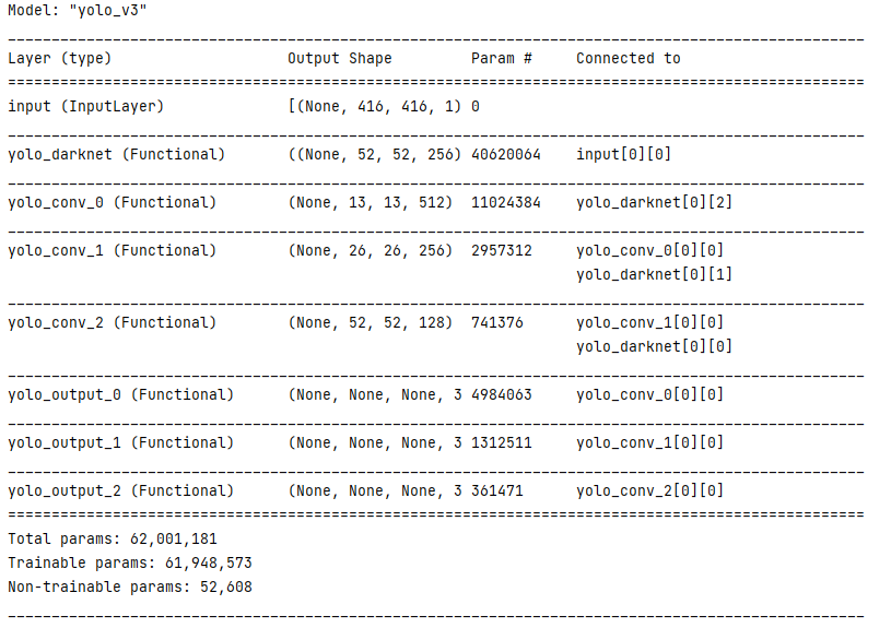
3.1.7,YoloV3

def YoloV3(size=None, channels=3, anchors=yolo_anchors,
           mask=yolo_anchor_masks, classes=80, training=False):
    x = inputs = Input([size, size, channels], name='input')

    x_8, x_16, x_32 = Darknet53(name='yolo_darknet')(x)

    x = YoloBlock(512, name='yolo_conv_0')(x_32)
    output_0 = YoloOutput(512, name='yolo_output_0')(x)

    x = YoloBlock(256, name='yolo_conv_1')((x, x_16))
    output_1 = YoloOutput(256, name='yolo_output_1')(x)

    x = YoloBlock(128, name='yolo_conv_2')((x, x_8))
    output_2 = YoloOutput(128, name='yolo_output_2')(x)
    return Model(inputs, (output_0, output_1, output_2), name='yolo_v3')

3.2 implementation of YOLOV3 loss

iou can use giou, diou, or ciou

3.2.1,iou

def box_iou(box_1, box_2):
    """

    :param box_1:  (..., (x1, y1, x2, y2))
    :param box_2: (N, (x1, y1, x2, y2))
    :return:  (N, 1)
    """

    # broadcast boxes
    box_1 = tf.expand_dims(box_1, -2)
    box_2 = tf.expand_dims(box_2, 0)
    # new_shape: (..., N, (x1, y1, x2, y2))
    new_shape = tf.broadcast_dynamic_shape(tf.shape(box_1), tf.shape(box_2))
    box_1 = tf.broadcast_to(box_1, new_shape)
    box_2 = tf.broadcast_to(box_2, new_shape)

    # Calculate Union area
    int_w = tf.maximum(tf.minimum(box_1[..., 2], box_2[..., 2]) -
                       tf.maximum(box_1[..., 0], box_2[..., 0]), 0)
    int_h = tf.maximum(tf.minimum(box_1[..., 3], box_2[..., 3]) -
                       tf.maximum(box_1[..., 1], box_2[..., 1]), 0)

    int_area = int_w * int_h
    # Calculate the area of two boxes
    box_1_area = (box_1[..., 2] - box_1[..., 0]) * \
        (box_1[..., 3] - box_1[..., 1])
    box_2_area = (box_2[..., 2] - box_2[..., 0]) * \
        (box_2[..., 3] - box_2[..., 1])
    # The intersection area is the area of two boxes and - Union area
    union_area = box_1_area + box_2_area - int_area
    # iou = intersection area / Union area, add epsilon in denominator to avoid dividing by 0
    iou = int_area / (union_area + tf.keras.backend.epsilon())

    return iou

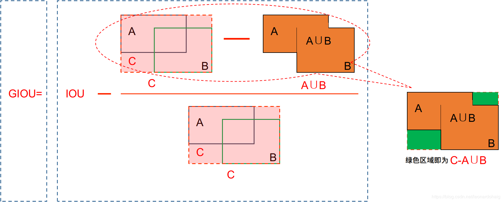
3.2.2,giou

giou solves the problem that the loss cannot be measured when two frames do not intersect (iou equals zero)

For intersecting frames, IOU can be back propagated, that is, it can be directly used as the objective function of optimization. But for non intersecting, the gradient will be 0 and cannot be optimized. Using GIoU at this time can completely avoid this problem. So it can be used as the objective function

def box_giou(box_1, box_2):
    """
    :param box_1:  (..., (x1, y1, x2, y2))
     :param box_2: (N, (x1, y1, x2, y2))
    :return:  (N, 1)
    """

    # broadcast boxes
    box_1 = tf.expand_dims(box_1, -2)
    box_2 = tf.expand_dims(box_2, 0)
    # new_shape: (..., N, (x1, y1, x2, y2))
    new_shape = tf.broadcast_dynamic_shape(tf.shape(box_1), tf.shape(box_2))
    box_1 = tf.broadcast_to(box_1, new_shape)
    box_2 = tf.broadcast_to(box_2, new_shape)
    # Calculate Union area
    intersect_w = tf.maximum(tf.minimum(box_1[..., 2], box_2[..., 2]) -
                       tf.maximum(box_1[..., 0], box_2[..., 0]), 0)
    intersect_h = tf.maximum(tf.minimum(box_1[..., 3], box_2[..., 3]) -
                       tf.maximum(box_1[..., 1], box_2[..., 1]), 0)
    intersect_area = intersect_w * intersect_h
    # Calculate the area of two boxes
    box_1_area = (box_1[..., 2] - box_1[..., 0]) * \
        (box_1[..., 3] - box_1[..., 1])
    box_2_area = (box_2[..., 2] - box_2[..., 0]) * \
        (box_2[..., 3] - box_2[..., 1])
    # The intersection area is the area of two boxes and - Union area
    union_area = box_1_area + box_2_area - intersect_area
    # iou = intersection area / Union area, add epsilon in denominator to avoid dividing by 0
    iou = intersect_area / (union_area + tf.keras.backend.epsilon())
    # Calculates the area of a rectangle surrounding two boxes
    enclose_w = tf.maximum(tf.maximum(box_1[..., 2], box_2[..., 2]) -
                       tf.minimum(box_1[..., 0], box_2[..., 0]), 0)
    enclose_h = tf.maximum(tf.maximum(box_1[..., 3], box_2[..., 3]) -
                       tf.minimum(box_1[..., 1], box_2[..., 1]), 0)
    enclose_area = enclose_w * enclose_h
    #giou = iou - (minimum bounding rectangle area intersection area) / minimum bounding rectangle area
    giou = iou - 1.0 * (enclose_area - union_area) / (enclose_area + tf.keras.backend.epsilon())

    return giou

3.2.3,diou

There are also problems with giou. If there are situations as shown in the figure below, giou will degenerate into iou

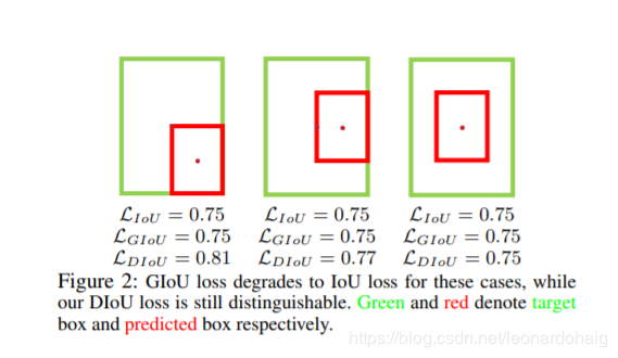
Consider another way to measure the distance between the two boxes

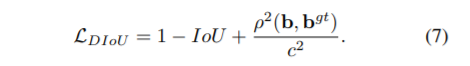
b. bgt represents the center points of anchor frame and target frame respectively, and p represents the Euclidean distance between the two center points. c represents the diagonal distance of the smallest rectangle that can cover both anchor and target box.

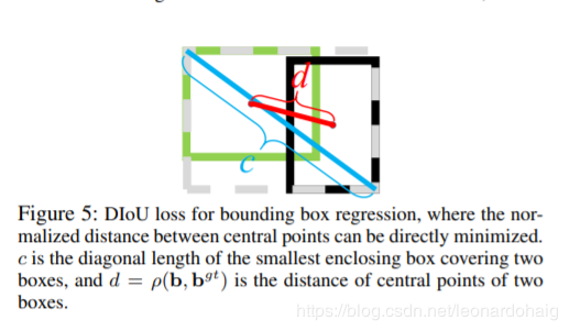
Similar to GIoU loss, DIoU loss can still provide the moving direction for the bounding box when it does not overlap with the target box.

DIoU loss can directly minimize the distance between two target boxes, while GIOU loss optimizes the area between two target boxes

def box_diou(box_1, box_2):
    """
    :param box_1:  (..., (x1, y1, x2, y2))
    :param box_2: (N, (x1, y1, x2, y2))
    :return:  (N, 1)
    """
    # broadcast boxes
    box_1 = tf.expand_dims(box_1, -2)
    box_2 = tf.expand_dims(box_2, 0)
    # new_shape: (..., N, (x1, y1, x2, y2))
    new_shape = tf.broadcast_dynamic_shape(tf.shape(box_1), tf.shape(box_2))
    box_1 = tf.broadcast_to(box_1, new_shape)
    box_2 = tf.broadcast_to(box_2, new_shape)
    # Calculate Union area
    intersect_w = tf.maximum(tf.minimum(box_1[..., 2], box_2[..., 2]) -
                             tf.maximum(box_1[..., 0], box_2[..., 0]), 0)
    intersect_h = tf.maximum(tf.minimum(box_1[..., 3], box_2[..., 3]) -
                             tf.maximum(box_1[..., 1], box_2[..., 1]), 0)
    intersect_area = intersect_w * intersect_h
    # Calculate the area of two boxes
    box_1_area = (box_1[..., 2] - box_1[..., 0]) * \
                 (box_1[..., 3] - box_1[..., 1])
    box_2_area = (box_2[..., 2] - box_2[..., 0]) * \
                 (box_2[..., 3] - box_2[..., 1])
    # The intersection area is the area of two boxes and - Union area
    union_area = box_1_area + box_2_area - intersect_area
    # iou = intersection area / Union area, add epsilon in denominator to avoid dividing by 0
    iou = intersect_area / (union_area + tf.keras.backend.epsilon())
    # The minimum diagonal of the rectangle w * h is calculated by the square of the rectangle w * H
    enclose_w = tf.maximum(tf.maximum(box_1[..., 2], box_2[..., 2]) -
                           tf.minimum(box_1[..., 0], box_2[..., 0]), 0)
    enclose_h = tf.maximum(tf.maximum(box_1[..., 3], box_2[..., 3]) -
                           tf.minimum(box_1[..., 1], box_2[..., 1]), 0)
    enclose_wh = tf.stack((enclose_w, enclose_h), axis=-1)
    enclose_diagonal = tf.keras.backend.sum(tf.square(enclose_wh), axis=-1)
    # Calculate the Euclidean distance between two center points and square it
    box_1_xy =  (box_1[..., 0:2] + box_1[..., 2:4]) / 2.0
    box_2_xy = (box_2[..., 0:2] + box_2[..., 2:4]) / 2.0
    center_distance = tf.keras.backend.sum(tf.square(box_1_xy - box_2_xy), axis=-1)
    # diou , add epsilon in denominator to avoid dividing by 0
    diou = iou - 1.0 * (center_distance) / (enclose_diagonal + tf.keras.backend.epsilon())

    return diou

3.2.4,ciou

A good target frame regression loss should consider three important geometric factors: overlapping area, center point distance and aspect ratio. GIoU: in order to normalize the coordinate scale, IoU is used and the case where IoU is zero is preliminarily solved. DIoU: DIoU loss considers both the overlapping area of the bounding box and the distance from the center point. CIOU: complete IoU loss, the consistency of the aspect ratio between the anchor box and the target box is also extremely important.

CIOU Loss also introduces a penalty term of box aspect ratio. The Loss considers the aspect ratio of box and is defined as follows:

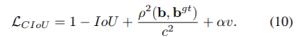
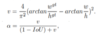
among α Is the parameter used to balance the scale. v is used to measure the proportion consistency between anchor box and target box. from α It can be seen from the definition of parameters that the loss function will be more inclined to optimize in the direction of increasing overlapping areas, especially when IoU is zero.

def box_ciou(box_1, box_2):
    """
    :param box_1:  (..., (x1, y1, x2, y2))
    :param box_2: (N, (x1, y1, x2, y2))
    :return:  (N, 1)
    """
    box_1 = tf.expand_dims(box_1, -2)
    box_2 = tf.expand_dims(box_2, 0)
    # new_shape: (..., N, (x1, y1, x2, y2))
    new_shape = tf.broadcast_dynamic_shape(tf.shape(box_1), tf.shape(box_2))
    box_1 = tf.broadcast_to(box_1, new_shape)
    box_2 = tf.broadcast_to(box_2, new_shape)
    # Calculate Union area
    intersect_w = tf.maximum(tf.minimum(box_1[..., 2], box_2[..., 2]) -
                             tf.maximum(box_1[..., 0], box_2[..., 0]), 0)
    intersect_h = tf.maximum(tf.minimum(box_1[..., 3], box_2[..., 3]) -
                             tf.maximum(box_1[..., 1], box_2[..., 1]), 0)
    intersect_area = intersect_w * intersect_h
    # Calculate the area of two boxes
    box_1_area = (box_1[..., 2] - box_1[..., 0]) * \
                 (box_1[..., 3] - box_1[..., 1])
    box_2_area = (box_2[..., 2] - box_2[..., 0]) * \
                 (box_2[..., 3] - box_2[..., 1])
    # The intersection area is the area of two boxes and - Union area
    union_area = box_1_area + box_2_area - intersect_area
    # iou = intersection area / Union area, add epsilon in denominator to avoid dividing by 0
    iou = intersect_area / (union_area + tf.keras.backend.epsilon())
    # Euclidean distance square of the center point of two frames
    box_1_xy = (box_1[..., 0:2] + box_1[..., 2:4]) / 2.0
    box_2_xy = (box_2[..., 0:2] + box_2[..., 2:4]) / 2.0
    center_distance = tf.keras.backend.sum(tf.square(box_1_xy - box_2_xy), axis=-1)
    # Calculate the minimum rectangle w, h surrounding the two boxes and the diagonal distance w*w + h*h of the minimum rectangle
    enclose_w = tf.maximum(tf.maximum(box_1[..., 2], box_2[..., 2]) -
                           tf.minimum(box_1[..., 0], box_2[..., 0]), 0)
    enclose_h = tf.maximum(tf.maximum(box_1[..., 3], box_2[..., 3]) -
                           tf.minimum(box_1[..., 1], box_2[..., 1]), 0)
    enclose_wh = tf.stack((enclose_w, enclose_h), axis=-1)
    # Calculate the minimum rectangle w, h surrounding the two boxes, and square the diagonal distance of the minimum rectangle w*w + h*h
    enclose_diagonal = tf.keras.backend.sum(tf.square(enclose_wh), axis=-1)
    # diou
    diou = iou - 1.0 * (center_distance) / (enclose_diagonal + tf.keras.backend.epsilon())

    box_1_w = (box_1[..., 2] - box_1[..., 0])
    box_1_h = (box_1[..., 3] - box_1[..., 1])
    box_2_w = (box_2[..., 2] - box_2[..., 0])
    box_2_h = (box_2[..., 3] - box_2[..., 1])

    v = 4 * tf.keras.backend.square(
        tf.math.atan2(box_1_w, box_1_h) - tf.math.atan2(box_2_w, box_2_h)) / (math.pi * math.pi)
    alpha = v / (1.0 - iou + v)
    # ciou
    ciou = diou - alpha * v

    return ciou

3.2.5,Loss

def yolo_boxes(pred, anchors, classes):
    # pred: (batch_size, grid, grid, anchors, (x, y, w, h, obj, ...classes))
    grid_size = tf.shape(pred)[1:3]

    # Split the last dimension XY wh obj classes (2, 2, 1, classes)
    box_xy, box_wh, objectness, class_probs = tf.split(pred, (2, 2, 1, classes), axis=-1)
    pred_box = tf.concat((box_xy, box_wh), axis=-1)

    # grid[x][y] == (y, x)

    grid = tf.meshgrid(tf.range(grid_size[1]), tf.range(grid_size[0]))
    grid = tf.expand_dims(tf.stack(grid, axis=-1), axis=2)

    """
    use sidmoid The function is forcibly restricted between 0 and 1
    bx = simmoid(tx) + Cx  by = simmoid(ty) + Cy 
    bw = pw*exp(tw)        bh = pw*exp(th)
    bx, by, bw, bh Center coordinate of prediction
    tx, ty, tw, th Network output
    Cx, Cy         Coordinates of the grid from top to left
    ph, pw         Height and width of a priori frame
    """

    box_xy = tf.sigmoid(box_xy)
    box_xy = (box_xy + tf.cast(grid, tf.float32))
    box_wh = tf.exp(box_wh) * anchors

    # Convert the upper left coordinate to relative coordinate
    box_xy = box_xy / tf.cast(grid_size, tf.float32)

    # Calculate the upper left and lower right coordinates
    box_x1y1 = box_xy - box_wh / 2
    box_x2y2 = box_xy + box_wh / 2
    bbox = tf.concat([box_x1y1, box_x2y2], axis=-1)

    objectness = tf.sigmoid(objectness)
    class_probs = tf.sigmoid(class_probs)


    return bbox, objectness, class_probs, pred_box

def yolo_boxes(pred, anchors, classes):
    # PRED: (batch_size, grid, grid, anchors, (x, y, W, h, obj,... Classes)) x, y, W, H predicted center coordinates and length and width
    grid_size = tf.shape(pred)[1:3]

    # Split the last dimension XY wh obj classes (2, 2, 1, classes)
    box_xy, box_wh, objectness, class_probs = tf.split(pred, (2, 2, 1, classes), axis=-1)
    pred_box = tf.concat((box_xy, box_wh), axis=-1)

    # grid[x][y] == (y, x)

    grid = tf.meshgrid(tf.range(grid_size[1]), tf.range(grid_size[0]))
    grid = tf.expand_dims(tf.stack(grid, axis=-1), axis=2)

    """
    use sidmoid The function is forcibly restricted between 0 and 1
    bx = simmoid(tx) + Cx  by = simmoid(ty) + Cy 
    bw = pw*exp(tw)        bh = pw*exp(th)
    bx, by, bw, bh Predicted center coordinates and length and width
    tx, ty, tw, th Output center coordinates and length and width of the network
    Cx, Cy         Coordinates of the grid from top to left
    ph, pw         Height and width of a priori frame
    """

    box_xy = tf.sigmoid(box_xy)
    box_xy = (box_xy + tf.cast(grid, tf.float32))
    box_wh = tf.exp(box_wh) * anchors

    # Convert center coordinates to relative coordinates
    box_xy = box_xy / tf.cast(grid_size, tf.float32)

    # Calculate the upper left and lower right coordinates
    box_x1y1 = box_xy - box_wh / 2
    box_x2y2 = box_xy + box_wh / 2
    bbox = tf.concat([box_x1y1, box_x2y2], axis=-1)
    # Confidence
    objectness = tf.sigmoid(objectness)
    # category
    class_probs = tf.sigmoid(class_probs)


    return bbox, objectness, class_probs, pred_box


def all_loss(args, anchors, masks):
    # Calculate the loss of the third floor
    yolo_outputs = args[:3]
    y_true = args[3:]
    lossFun = [YoloLoss(anchors[mask], classes=80) for mask in masks]

    loss = 0
    for i, l in enumerate(lossFun):
        loss += l(y_true[i], yolo_outputs[i])

    return loss

3.3 data input

3.3.1,K-meas

The k-means algorithm needs to input the data to be clustered and the number of clusters to be clustered K. The main process is as follows:
1. Randomly generate K initial points as centroids
2. Centralize the data according to the distance from the far center of mass to the near center of mass
3. Average the data in each cluster as a new centroid and repeat the previous step until all clusters do not change

import numpy as np
from config import *


class YOLO_Kmeans:

    def __init__(self, cluster_number, filename, anchor_save):
        self.cluster_number = cluster_number
        self.filename = filename
        self.anchor_save = anchor_save

    def iou(self, boxes, clusters):  # 1 box -> k clusters
        n = boxes.shape[0]
        k = self.cluster_number

        box_area = boxes[:, 0] * boxes[:, 1]
        box_area = box_area.repeat(k)
        box_area = np.reshape(box_area, (n, k))

        cluster_area = clusters[:, 0] * clusters[:, 1]
        cluster_area = np.tile(cluster_area, [1, n])
        cluster_area = np.reshape(cluster_area, (n, k))

        box_w_matrix = np.reshape(boxes[:, 0].repeat(k), (n, k))
        cluster_w_matrix = np.reshape(np.tile(clusters[:, 0], (1, n)), (n, k))
        min_w_matrix = np.minimum(cluster_w_matrix, box_w_matrix)

        box_h_matrix = np.reshape(boxes[:, 1].repeat(k), (n, k))
        cluster_h_matrix = np.reshape(np.tile(clusters[:, 1], (1, n)), (n, k))
        min_h_matrix = np.minimum(cluster_h_matrix, box_h_matrix)
        inter_area = np.multiply(min_w_matrix, min_h_matrix)

        result = inter_area / (box_area + cluster_area - inter_area)
        return result

    def avg_iou(self, boxes, clusters):
        accuracy = np.mean([np.max(self.iou(boxes, clusters), axis=1)])
        return accuracy

    def kmeans(self, boxes, k, dist=np.median):
        box_number = boxes.shape[0]
        distances = np.empty((box_number, k))
        last_nearest = np.zeros((box_number,))
        np.random.seed()
        clusters = boxes[np.random.choice(
            box_number, k, replace=False)]  # init k clusters
        while True:

            distances = 1 - self.iou(boxes, clusters)

            current_nearest = np.argmin(distances, axis=1)
            if (last_nearest == current_nearest).all():
                break  # clusters won't change
            for cluster in range(k):
                clusters[cluster] = dist(  # update clusters
                    boxes[current_nearest == cluster], axis=0)

            last_nearest = current_nearest

        return clusters

    def result2txt(self, data):
        f = open(self.anchor_save, 'w')
        row = np.shape(data)[0]
        for i in range(row):
            if i == 0:
                x_y = "%d,%d" % (data[i][0], data[i][1])
            else:
                x_y = ", %d,%d" % (data[i][0], data[i][1])
            f.write(x_y)
        f.close()

    def txt2boxes(self):
        f = open(self.filename, 'r')
        dataSet = []
        for line in f:
            infos = line.split(" ")
            length = len(infos)
            for i in range(1, length):
                width = int(infos[i].split(",")[2]) - \
                        int(infos[i].split(",")[0])
                height = int(infos[i].split(",")[3]) - \
                         int(infos[i].split(",")[1])
                dataSet.append([width, height])
        result = np.array(dataSet)
        f.close()
        return result

    def txt2clusters(self):
        all_boxes = self.txt2boxes()
        result = self.kmeans(all_boxes, k=self.cluster_number)
        result = result[np.lexsort(result.T[0, None])]
        self.result2txt(result)
        print("K anchors:\n {}".format(result))
        print("Accuracy: {:.2f}%".format(
            self.avg_iou(all_boxes, result) * 100))


if __name__ == "__main__":
    cluster_number = 2
    filename = "./train_file/train.txt"
    anchor_save = "./train_anchor/anchors.txt"
    kmeans = YOLO_Kmeans(cluster_number, filename, anchor_save)
    kmeans.txt2clusters()

3.3.2,data_generator

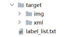
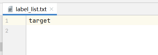
My dataset file is as follows: target is a target, which contains two folders img to store pictures, xml files and label_list.txt is the category name

import numpy as np
import tensorflow as tf
import os
import cv2 as cv
import xml.etree.ElementTree as ET


def transform_images(x_train, size):
    # Crop the image size and normalize it
    x_train = tf.image.resize(x_train, (size, size)) / 255.0
    return x_train


def preprocess_true_boxes(true_boxes, input_shape, anchors, num_classes):
    """
    Preprocess true boxes to training input format
    Args:
        true_boxes: array, shape=(m, T, 5) relative x_min, y_min, x_max, y_max, class_id .
        input_shape: array-like, hw, multiples of 32
        anchors: array, shape=(N, 2), wh
        num_classes: integer

    Returns:
        y_true: list of array, shape like yolo_outputs, xywh are reletive value

    """
    assert (true_boxes[..., 4] < num_classes).all(), 'class id must be less than num_classes'
    num_layers = len(anchors) // 3  # default setting

    anchor_mask = [[6, 7, 8], [3, 4, 5], [0, 1, 2]] if num_layers == 3 else [[3, 4, 5], [1, 2, 3]]

    true_boxes = np.array(true_boxes, dtype='float32')
    input_shape = np.array(input_shape, dtype='int32')
    # boxes_xy = (true_boxes[..., 0:2] + true_boxes[..., 2:4]) // 2 # center point coordinates
    boxes_wh = true_boxes[..., 2:4] - true_boxes[..., 0:2]  # w，h
    # true_boxes[..., 0:2] = boxes_xy / input_shape[::-1]  # Relative coordinates
    # true_boxes[..., 2:4] = boxes_wh / input_shape[::-1]

    m = true_boxes.shape[0]
    grid_shapes = [input_shape // {0: 32, 1: 16, 2: 8}[l] for l in range(num_layers)]
    y_true = [np.zeros((m, grid_shapes[l][0], grid_shapes[l][1], len(anchor_mask[l]), 5 + num_classes),
                       dtype='float32') for l in range(num_layers)]

    # Expand dim to apply broadcasting.
    anchors = np.expand_dims(anchors, 0)
    anchor_maxes = anchors / 2.
    anchor_mins = -anchor_maxes
    valid_mask = boxes_wh[..., 0] > 0

    for b in range(m):
        # Discard zero rows.
        wh = boxes_wh[b, valid_mask[b]]
        if len(wh) == 0: continue
        # Expand dim to apply broadcasting.
        wh = np.expand_dims(wh, -2)
        box_maxes = wh / 2.
        box_mins = -box_maxes

        intersect_mins = np.maximum(box_mins, anchor_mins)
        intersect_maxes = np.minimum(box_maxes, anchor_maxes)
        intersect_wh = np.maximum(intersect_maxes - intersect_mins, 0.)
        intersect_area = intersect_wh[..., 0] * intersect_wh[..., 1]
        box_area = wh[..., 0] * wh[..., 1]
        anchor_area = anchors[..., 0] * anchors[..., 1]
        iou = intersect_area / (box_area + anchor_area - intersect_area)

        # Find best anchor for each true box
        best_anchor = np.argmax(iou, axis=-1)

        for t, n in enumerate(best_anchor):
            for l in range(num_layers):
                if n in anchor_mask[l]:
                    i = np.floor(true_boxes[b, t, 0] * grid_shapes[l][1]).astype('int32')
                    j = np.floor(true_boxes[b, t, 1] * grid_shapes[l][0]).astype('int32')
                    k = anchor_mask[l].index(n)
                    c = true_boxes[b, t, 4].astype('int32')
                    y_true[l][b, j, i, k, 0:4] = true_boxes[b, t, 0:4]
                    y_true[l][b, j, i, k, 4] = 1
                    # The confidence level is 1, indicating that there is an object ont hot coding
                    y_true[l][b, j, i, k, 5 + c] = 1
    # 3 x [batchsize, grid, grid, 3, 25]
    '''
    :return
    grid:       In which grid What point is output
    3   :       Which set anchor，There are three sets in total, three for each set anchor，grid=13x13，It corresponds to the first set
    25  :       0-4 Represents a relative value based on 416
    '''
    return y_true



def get_data_from_file(path, yolo_anchors, max_box_num, input_szie):
    assert os.path.isdir(path), "The path does not exist"
    label_list = [label_name.strip() for label_name in open(os.path.join(path + 'label_list.txt')).readlines()]
    num_classes = len(label_list)
    all_data_image = []
    all_data_label = []
    dirs = [os.path.join(path,filename) for filename in os.listdir(path) if os.path.isdir(path + filename)]

    for dirname in dirs:
        for data_dir_file in os.listdir(dirname):
            if data_dir_file == "img":
                data_dir_file = os.path.join(dirname, data_dir_file)
                for img_filename in os.listdir(data_dir_file):
                    img = cv.imread(os.path.join(data_dir_file, img_filename))
                    # Picture normalization
                    img = cv.resize(img, (input_szie, input_szie)) / 255.0
                    all_data_image.append(img)

            if data_dir_file == "xml":
                data_dir_file = os.path.join(dirname, data_dir_file)
                xml_filenames = [xml_filename for xml_filename in os.listdir(data_dir_file) if xml_filename.endswith("xml")]
                for xml_filename in xml_filenames:
                    tree = ET.parse(os.path.join(data_dir_file, xml_filename))
                    root = tree.getroot()
                    boxes_list = []
                    width =  int(root.find("size")[0].text)
                    height = int(root.find("size")[1].text)
                    for object in root.findall("object"):
                        labelname = object[0].text
                        # Convert to relative coordinates
                        xmin = int(object[4][0].text) / width
                        ymin = int(object[4][1].text) / height
                        xmax = int(object[4][2].text) / width
                        ymax = int(object[4][3].text) / height
                        label = label_list.index(labelname)
                        boxes_list.append(np.array((xmin, ymin, xmax, ymax, label)).astype(np.float64))
                    boxes_arr = np.stack(boxes_list)
                    paddings = [[0, max_box_num - np.shape(boxes_arr)[0]], [0, 0]]
                    boxes = np.pad(boxes_arr, paddings)
                    all_data_label.append(boxes)

    all_data_image = np.stack(all_data_image, axis=0)
    all_data_label = np.stack(all_data_label, axis=0)
    # Data of three different sizes
    all_data_label = preprocess_true_boxes(all_data_label, (input_szie, input_szie), yolo_anchors, num_classes)

    return all_data_image, all_data_label


def draw_box(img, classes):
    boxes, classid = classes[..., 0:4], classes[..., 4:]

    img_size = np.array((img.shape[1], img.shape[0]))
    for i in range(len(boxes)):
        print(boxes[i])
        x1y1 = tuple(((np.array(boxes[i][0:2])) * img_size).astype(np.int32))
        print(x1y1)
        x2y2 = tuple(((np.array(boxes[i][2:4])) * img_size).astype(np.int32))
        img = cv.rectangle(img, x1y1, x2y2, (255, 0, 0), 2)
        img = cv.putText(img, '{}'.format(classid[i]),x1y1, cv.FONT_HERSHEY_COMPLEX_SMALL, 1, (0, 0, 255), 2)
    cv.imshow("box", img)
    cv.waitKey()


class DatasetGenerator():
    def __init__(self, datas, shuffle, batch_size):
        self._shuffle = shuffle
        self._batch_size = batch_size
        self._indicator = 0
        self._data = datas[0]

        self._labels_13 = datas[1][0]
        self._labels_26 = datas[1][1]
        self._labels_52 = datas[1][2]

        self.count = self._data.shape[0]

    def __iter__(self):
        return self

    def __next__(self):
        return self._next_batch()

    def _shuffle_data(self):
        p = np.random.permutation(self.count)
        self._data = self._data[p]
        self._labels_13 = self._labels_13[p]
        self._labels_26 = self._labels_26[p]
        self._labels_52 = self._labels_52[p]

    def _next_batch(self):
        end_indicator = self._indicator + self._batch_size

        if end_indicator > self.count:
            if self._shuffle:
                self._shuffle_data()
                self._indicator = 0
                end_indicator = self._batch_size
            else:
                self._indicator = 0
                end_indicator = self._batch_size

        if end_indicator > self.count:
            raise StopIteration
        batch_data = self._data[self._indicator: end_indicator]
        batch_labels_13 = self._labels_13[self._indicator: end_indicator]
        batch_labels_26 = self._labels_26[self._indicator: end_indicator]
        batch_labels_52 = self._labels_52[self._indicator: end_indicator]
        self._indicator = end_indicator

        return batch_data, (batch_labels_13, batch_labels_26, batch_labels_52)

3.4 network training

def setup_model(num_classes, lreaning_rate):
    model = YoloV3(416, training=True,
                   classes=num_classes)

    anchors = yolo_anchors
    anchor_masks = yolo_anchor_masks

    optimizer = tf.keras.optimizers.Adam(lr=lreaning_rate)
    loss = [YoloLoss(anchors[mask], num_classes=num_classes) for mask in anchor_masks]

    model.summary()
    model.compile(optimizer=optimizer, loss=loss)

    return model, loss


def main():
    input_size = 416      # Enter picture size
    learning_rate = 1e-4  # Learning rate
    batch_size = 8        # Data size of each batch
    epochs = 100          # Total training rounds
    num_classes = 1       # Number of categories
    datafile = "./data/"  # Dataset path
    max_box_num = 100     # Maximum number of targets in a picture
    model_filepath = "./model_filepath/"                            # Model save location
    checkpoint_filepath = model_filepath + "checkpoint_filepath/"   # Weight save location
    log_path = model_filepath + "log_path/"                         # Log file save location

    datas = get_data_from_file(datafile, yolo_anchors, max_box_num, input_size)
    trianGenerator = DatasetGenerator(datas, True, batch_size)
    use_gpu = True

    if use_gpu:
        gpus = tf.config.experimental.list_physical_devices(device_type='GPU')
        if gpus:
            for gpu in gpus:
                tf.config.experimental.set_memory_growth(device=gpu, enable=True)
                tf.print(gpu)

        else:
            os.environ["CUDA_VISIBLE_DEVICE"] = "-1"

    else:
        os.environ["CUDA_VISIBLE_DEVICE"] = "-1"

    cp_callback = tf.keras.callbacks.ModelCheckpoint(
        filepath=checkpoint_filepath,  # File path
        save_best_only=True,           # Best preserved
        save_weights_only=True,        # Save parameters only
        monitor='loss',                # Value to monitor
        mode='auto',                   # pattern
        period=1,                      # The number of epoch s in the interval between checkpoints
    )
    log = tf.keras.callbacks.TensorBoard(log_dir=log_path)
    model, loss = setup_model(num_classes, learning_rate)
    model.summary()
    history = model.fit(
        trianGenerator,
        epochs=epochs,
        steps_per_epoch=trianGenerator.count // batch_size + 1,
        callbacks=[cp_callback, log]
    )

    model.save()


if __name__ == '__main__':
    # try:
    #     app.run(main)
    # except SystemExit:
    #     pass
    main()

Visual training process

TensorBoard is a visual tool, which can be used to display network diagram, tensor index change, tensor distribution, etc. Enter the upper folder of the logging folder and run the command in the DOS window:

tensorboard --logdir=./log_path

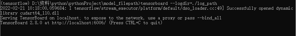
Enter the web address in the browser: http://localhost:6006 , or enter the URL prompted in the figure above to view the generated map.

3.5 network prediction

3.5.1 loading model

if __name__ == '__main__':
    input_size = 416

    learning_rate = 1e-5
    batch_size = 8

    model_filepath ="./model_filepath/"
    checkpoint_filepath = model_filepath + "checkpoint_filepath/"

    model = YoloV3(416, 1)

    model.load_weights(checkpoint_filepath)

    model.summary()

    img = cv2.imread("data/target/img/0.jpg")
    img = cv2.resize(img, (416, 416))
    img = np.expand_dims(img, axis=0)
    out = model.predict(img)

3.5.2,nms

def yolo_nms(outputs, classes):
    """
    :param outputs: list (bbox, objectness, class_probs)
    :param classes: int
    :return:
    """
    # boxes, conf, type
    b, c, t = [], [], []


    for o in outputs:
        boxes = o[..., 0:4]
        b.append(tf.reshape(boxes, (tf.shape(boxes)[0], -1, tf.shape(boxes)[-1])))
        conf  = o[..., 4:5]
        c.append(tf.reshape(conf, (tf.shape(conf)[0], -1, tf.shape(conf)[-1])))
        type  = o[..., 5:]
        t.append(tf.reshape(type, (tf.shape(type)[0], -1, tf.shape(type)[-1])))

    bbox = tf.concat(b, axis=1)           # (1, 13*13*3+26*26*3+52*52*3, 4)
    confidence = tf.concat(c, axis=1)     # (1, 13*13*3+26*26*3+52*52*3, 1)
    class_probs = tf.concat(t, axis=1)    # (1, 13*13*3+26*26*3+52*52*3, 80)


    if classes == 1:
        scores = confidence
    else:
        scores = confidence * class_probs # (1, 13*13*3+26*26*3+52*52*3, 80)
    # Delete 0 dimension
    dscores = tf.squeeze(scores, axis=0)  # (13*13*3+26*26*3+52*52*3, 80)
    scores = tf.reduce_max(dscores,[1])   # (13*13*3+26*26*3+52*52*3)
    bbox = tf.reshape(bbox, (-1, 4))      # (13*13*3+26*26*3+52*52*3, 4)
    classes = tf.argmax(dscores, 1)

    # Index, value
    selected_indices, selected_scores = tf.image.non_max_suppression_with_scores(
        boxes=bbox,
        scores=scores,
        max_output_size=100,
        iou_threshold=0.5,
        score_threshold=0.5,
        soft_nms_sigma=0.5
    )

    num_valid_nms_boxes = tf.shape(selected_indices)[0]
    selected_indices = tf.concat([selected_indices,tf.zeros(100-num_valid_nms_boxes, dtype=tf.int32)], 0)
    selected_scores = tf.concat([selected_scores, tf.zeros(100-num_valid_nms_boxes, dtype=tf.float32)], -1)


    boxes = tf.gather(bbox, selected_indices)
    boxes = tf.expand_dims(boxes, axis=0)
    scores = selected_scores
    scores = tf.expand_dims(scores, axis=0)
    classes = tf.gather(classes, selected_indices)
    classes = tf.expand_dims(classes, axis=0)
    valid_detections = num_valid_nms_boxes
    valid_detections = tf.expand_dims(valid_detections, axis=0)

    return boxes, scores, classes, valid_detections

3.5.3 draw box

def draw_box(img, classes):
    boxes, classid = classes[..., 0:4], classes[..., 4:]

    img_size = np.array((img.shape[1], img.shape[0]))
    for i in range(len(boxes)):
        print(boxes[i])
        x1y1 = tuple(((np.array(boxes[i][0:2])) * img_size).astype(np.int32))
        print(x1y1)
        x2y2 = tuple(((np.array(boxes[i][2:4])) * img_size).astype(np.int32))
        img = cv.rectangle(img, x1y1, x2y2, (255, 0, 0), 2)
        img = cv.putText(img, '{}'.format(classid[i]),x1y1, cv.FONT_HERSHEY_COMPLEX_SMALL, 1, (0, 0, 255), 2)
    cv.imshow("box", img)
    cv.waitKey()

4, opencv code implementation

Updating

reference resources

Original text of the paper: https://pjreddie.com/media/files/papers/YOLOv3.pdf
yolo details: https://blog.csdn.net/monk1992/article/details/82346138
Detailed analysis of YOLOv3 network structure: https://zhuanlan.zhihu.com/p/162043754
Detailed explanation of YOLOv3: https://www.jianshu.com/p/043966013dde
Interpretation of Yolo trilogy -- Yolov3: https://zhuanlan.zhihu.com/p/76802514
Darknet53 network structure and code implementation: https://blog.csdn.net/weixin_48167570/article/details/120688156
Phase I target detector - RetinaNet network understanding: https://zhuanlan.zhihu.com/p/410436667
Introduction to the concept of anchor box / prior bounding box and its generation: https://blog.csdn.net/qq_46110834/article/details/111410923
YOLOv3 data input: https://blog.csdn.net/weixin_42078618/article/details/85001224
Link 1: https://github.com/xiao9616/yolo4_tensorflow2
Link 2: https://github.com/zzh8829/yolov3-tf2