abstract
This example extracts part of the data in the plant seedling data set as the data set. The data set has 12 categories. Today, I work with you to implement tensorflow2 For the X version image classification task, the classification model uses MobileNetV1. The algorithm implemented in this paper has the following characteristics:
1. The image loading method is customized, which is more flexible and efficient. There is no need to load the image into memory at one time, which saves memory and is suitable for large-scale data sets.
2. Load the pre training weight of the model, and the training time is shorter.
3. For data enhancement, we choose evaluations.
For a more detailed explanation of MobileNetV1, please refer to the following articles:
https://blog.csdn.net/hhhhhhhhhhwwwwwwwwww/article/details/122699618
train
The first step is to import the required data package and set the global parameters
import numpy as np
from tensorflow.keras.optimizers import Adam
import cv2
from tensorflow.keras.preprocessing.image import img_to_array
from sklearn.model_selection import train_test_split
from tensorflow.python.keras.callbacks import ModelCheckpoint, ReduceLROnPlateau
from tensorflow.keras.applications import MobileNet
import os
import tensorflow as tf
from tensorflow.python.keras.layers import Dense
from tensorflow.python.keras.models import Sequential
import albumentations

norm_size = 224
datapath = 'data/train'
EPOCHS = 100
INIT_LR = 3e-4
labelList = []
dicClass = {'Black-grass': 0, 'Charlock': 1, 'Cleavers': 2, 'Common Chickweed': 3, 'Common wheat': 4, 'Fat Hen': 5, 'Loose Silky-bent': 6,
            'Maize': 7, 'Scentless Mayweed': 8, 'Shepherds Purse': 9, 'Small-flowered Cranesbill': 10, 'Sugar beet': 11}
classnum = 12
batch_size = 16
np.random.seed(42)
Here you can see tensorflow 2 Versions above 0 integrate keras. We don't need to install keras separately when using it. The previous code is upgraded to tensorflow2 For versions above 0, add tensorflow in front of keras.
After tensorflow is finished, let's explain some important global parameters:
-
norm_size = 224 sets the size of the input image. The default image size of MobileNet is 224 × 224.
-
datapath = 'data/train' set the path to store pictures. Here, it should be explained that if there are many pictures, they must not be placed in the project directory, otherwise pychar will browse all pictures when loading the project, which is very slow.
-
Epochs = the number of 100 epochs. The problem of how appropriate the setting of epochs is is very tangled. Generally, setting 300 is enough. If you feel that it is not well trained, load the model for training.
-
INIT_LR = 1e-3 learning rate. Generally, it gradually decreases from 0.001, and it should not be too small. It can be as small as 1e-6.
-
Classnum = number of 12 categories. The dataset has two categories, and all are divided into two categories.
-
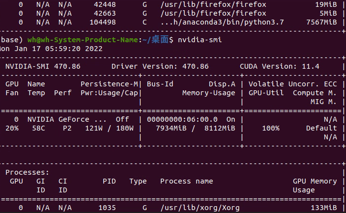
batch_size =16 batchsize. According to the hardware and the size of the data set, it is too small, the loss float is too large, and the convergence is not good. According to experience, it is generally set to the power of 2. windows can view the occupation of video memory through task manager.

Ubuntu can use NVIDIA SMI to check the occupation of video memory.
-
Define numpy Random factor of random. In this way, the random index can be fixed
Step 2: load pictures
Different from the previous practice, the image is no longer processed here, but only the list of image paths is returned.
See code for details:
def loadImageData():
    imageList = []
    listClasses = os.listdir(datapath)  # Category folder
    print(listClasses)
    for class_name in listClasses:
        label_id = dicClass[class_name]
        class_path = os.path.join(datapath, class_name)
        image_names = os.listdir(class_path)
        for image_name in image_names:
            image_full_path = os.path.join(class_path, image_name)
            labelList.append(label_id)
            imageList.append(image_full_path)
    return imageList


print("Start loading data")
imageArr = loadImageData()
labelList = np.array(labelList)
print("Loading data complete")
After making the data, we need to segment the training set and the test set, generally in the proportion of 4:1 or 7:3. Split dataset using train_test_split() method, import from sklearn model_ selection import train_ test_ Split package. Example:
trainX, valX, trainY, valY = train_test_split(imageArr, labelList, test_size=0.2, random_state=42)
Step 3 image enhancement
train_transform = albumentations.Compose([
        albumentations.OneOf([
            albumentations.RandomGamma(gamma_limit=(60, 120), p=0.9),
            albumentations.RandomBrightnessContrast(brightness_limit=0.2, contrast_limit=0.2, p=0.9),
            albumentations.CLAHE(clip_limit=4.0, tile_grid_size=(4, 4), p=0.9),
        ]),
        albumentations.HorizontalFlip(p=0.5),
        albumentations.ShiftScaleRotate(shift_limit=0.2, scale_limit=0.2, rotate_limit=20,
                                        interpolation=cv2.INTER_LINEAR, border_mode=cv2.BORDER_CONSTANT, p=1),
        albumentations.Normalize(mean=(0.485, 0.456, 0.406), std=(0.229, 0.224, 0.225), max_pixel_value=255.0, p=1.0)
    ])
val_transform = albumentations.Compose([
        albumentations.Normalize(mean=(0.485, 0.456, 0.406), std=(0.229, 0.224, 0.225), max_pixel_value=255.0, p=1.0)
    ])
For the specific settings, please refer to my previous articles:
Usage Summary of image enhancement Library_ AI Hao CSDN blog_ albumentations
Two data enhancements are written, one for training and one for verification. The verification set only needs to normalize the image.
Step 4 define the method of image processing
The main function of the generator is to process the image and return a batch image and the corresponding label in an iterative way.
Idea:
Loop in while:
-
Initialize input_samples and input_labels and a list are used to store the labels corresponding to image and image respectively.
-
Cyclic batch_size times:
-
- Random index
- From file_pathList and labels to get the path of the picture and the corresponding label
- Read picture
- If it is a training transform, it will be trained. If it is not, it will execute the verified transform.
- resize picture
- Convert image to array
- Put the image and label into input respectively_ Samples and input_labels
-
Convert list to numpy array.
-
Returns an iteration
def generator(file_pathList,labels,batch_size,train_action=False):
    L = len(file_pathList)
    while True:
        input_labels = []
        input_samples = []
        for row in range(0, batch_size):
            temp = np.random.randint(0, L)
            X = file_pathList[temp]
            Y = labels[temp]
            image = cv2.imdecode(np.fromfile(X, dtype=np.uint8), -1)
            if image.shape[2] > 3:
                image = image[:, :, :3]
            if train_action:
                image=train_transform(image=image)['image']
            else:
                image = val_transform(image=image)['image']
            image = cv2.resize(image, (norm_size, norm_size), interpolation=cv2.INTER_LANCZOS4)
            image = img_to_array(image)
            input_samples.append(image)
            input_labels.append(Y)
        batch_x = np.asarray(input_samples)
        batch_y = np.asarray(input_labels)
        yield (batch_x, batch_y)
The fifth step is to retain the best model and dynamically set the learning rate
Model checkpoint: used to save the best model.
The syntax is as follows:
keras.callbacks.ModelCheckpoint(filepath, monitor='val_loss', verbose=0, save_best_only=False, save_weights_only=False, mode='auto', period=1)
The callback function will save the model to filepath after each epoch
filepath can be a formatted string, and the placeholder inside will be passed in by the epoch value and on_ epoch_ The logs keyword of end
For example, if filepath is weights {epoch:02d-{val_loss:.2f}}. HDF5, multiple files corresponding to epoch and verification set loss will be generated.
parameter
- filename: string, the path to save the model
- monitor: the value to be monitored
- verbose: information display mode, 0 or 1
- save_best_only: when set to True, only the best performing models on the validation set will be saved
- Mode: one of 'auto', 'min' and 'Max', in save_ best_ When only = true, it determines the evaluation criteria of the best performance model, for example, when the monitoring value is val_acc, the mode should be max, when the detection value is val_ When loss, the mode should be min. In auto mode, the evaluation criteria are automatically inferred from the name of the monitored value.
- save_weights_only: if it is set to True, only the model weight will be saved, otherwise the whole model (including model structure, configuration information, etc.) will be saved
- period: the number of epoch s in the interval between checkpoints
Reducerlonplateau: when the evaluation index is not improving, reduce the learning rate. The syntax is as follows:
keras.callbacks.ReduceLROnPlateau(monitor='val_loss', factor=0.1, patience=10, verbose=0, mode='auto', epsilon=0.0001, cooldown=0, min_lr=0)
When learning stagnates, reducing the learning rate by 2 or 10 times can often achieve better results. This callback function detects the condition of the index. If the performance improvement of the model is not seen in the patient epoch s, the learning rate will be reduced
parameter
- monitor: monitored quantity
- Factor: the factor that reduces the learning rate each time. The learning rate will be reduced in the form of lr = lr*factor
- patience: when an epoch passes and the performance of the model does not improve, the action of reducing the learning rate will be triggered
- Mode: 'auto', 'min' and 'max'. In Min mode, if the detection value triggers the reduction of learning rate. In max mode, when the detection value no longer rises, the learning rate decreases.
- epsilon: threshold, used to determine whether to enter the "plain area" of the detection value
- Cooldown: after the learning rate decreases, the normal operation will be resumed after a cooldown epoch
- min_lr: lower limit of learning rate
The code of this example is as follows:
checkpointer = ModelCheckpoint(filepath='best_model.hdf5',
                               monitor='val_accuracy', verbose=1, save_best_only=True, mode='max')

reduce = ReduceLROnPlateau(monitor='val_accuracy', patience=10,
                           verbose=1,
                           factor=0.5,
                           min_lr=1e-6)
Step 6 establish the model and train
model = Sequential()
model.add(InceptionV3(include_top=False, pooling='avg', weights='imagenet'))
model.add(Dense(classnum, activation='softmax'))
optimizer = Adam(learning_rate=INIT_LR)
model.compile(optimizer=optimizer, loss='sparse_categorical_crossentropy', metrics=['accuracy'])
history = model.fit(generator(trainX,trainY,batch_size,train_action=True),
                              steps_per_epoch=len(trainX) / batch_size,
                              validation_data=generator(valX,valY,batch_size,train_action=False),
                              epochs=EPOCHS,
                              validation_steps=len(valX) / batch_size,
                              callbacks=[checkpointer, reduce])
model.save('my_model.h5')
print(history)
The pre training model was not used in the previous blog post. There was an error in the use of this post. After consulting the data, it was found that this method is wrong, as follows:
#model = MobileNet(weights="imagenet",input_shape=(224,224,3),include_top=False, classes=classnum) #include_top=False remove the last full connection layer
If you want to specify classes, there are two conditions: include_top: True, weights: None. Otherwise, you cannot specify classes.
Therefore, pre training cannot be used to specify classes, so another method is adopted:
model = Sequential()
model.add(MobileNet(include_top=False, pooling='avg', weights='imagenet'))
model.add(Dense(classnum, activation='softmax'))
In addition, the last article used fit_generator. In the new version, fit supports the generator mode, so it is changed to fit.
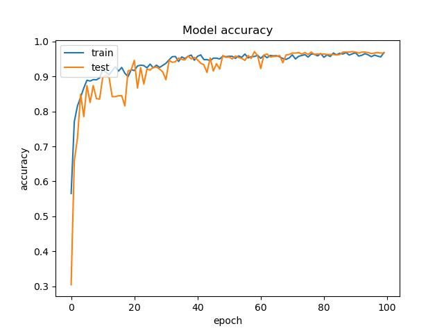
Step 7 keep the training results and generate pictures
loss_trend_graph_path = r"WW_loss.jpg"
acc_trend_graph_path = r"WW_acc.jpg"
import matplotlib.pyplot as plt
print("Now,we start drawing the loss and acc trends graph...")
# summarize history for accuracy
fig = plt.figure(1)
plt.plot(history.history["accuracy"])
plt.plot(history.history["val_accuracy"])
plt.title("Model accuracy")
plt.ylabel("accuracy")
plt.xlabel("epoch")
plt.legend(["train", "test"], loc="upper left")
plt.savefig(acc_trend_graph_path)
plt.close(1)
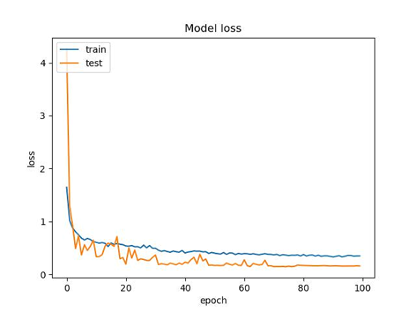
# summarize history for loss
fig = plt.figure(2)
plt.plot(history.history["loss"])
plt.plot(history.history["val_loss"])
plt.title("Model loss")
plt.ylabel("loss")
plt.xlabel("epoch")
plt.legend(["train", "test"], loc="upper left")
plt.savefig(loss_trend_graph_path)
plt.close(2)
print("We are done, everything seems OK...")
# #windows system setting 10 shutdown
#os.system("shutdown -s -t 10")
Test part
Single picture prediction
1. Import dependency
import cv2
import numpy as np
from tensorflow.keras.preprocessing.image import img_to_array
from  tensorflow.keras.models import load_model
import time
import os
import albumentations
2. Set global parameters
Note here that the order of the dictionary is consistent with that of the training
norm_size=224
imagelist=[]
emotion_labels = {
    0: 'Black-grass',
    1: 'Charlock',
    2: 'Cleavers',
    3: 'Common Chickweed',
    4: 'Common wheat',
    5: 'Fat Hen',
    6: 'Loose Silky-bent',
    7: 'Maize',
    8: 'Scentless Mayweed',
    9: 'Shepherds Purse',
    10: 'Small-flowered Cranesbill',
    11: 'Sugar beet',
}
3. Set picture normalization parameters
The setting of normalization parameters is consistent with the verified parameters
val_transform = albumentations.Compose([
        albumentations.Normalize(mean=(0.485, 0.456, 0.406), std=(0.229, 0.224, 0.225), max_pixel_value=255.0, p=1.0)
    ])
3. Loading model
emotion_classifier=load_model("my_model.h5")
4. Processing pictures
The logic of processing pictures is similar to that of training sets. The steps are as follows:
- Read picture
- resize the picture to norm_size × norm_size.
- Convert the picture to an array.
- Put it in the imagelist.
- Convert list to numpy array.
image = cv2.imdecode(np.fromfile('data/test/0a64e3e6c.png', dtype=np.uint8), -1)
image = val_transform(image=image)['image']
image = cv2.resize(image, (norm_size, norm_size), interpolation=cv2.INTER_LANCZOS4)
image = img_to_array(image)
imagelist.append(image)
imageList = np.array(imagelist, dtype="float")
5. Forecast category
Predict the category and get the index of the highest category.
pre=np.argmax(emotion_classifier.predict(imageList))
emotion = emotion_labels[pre]
t2=time.time()
print(emotion)
t3=t2-t1
print(t3)
Batch forecast
The difference between batch forecast and single sheet forecast mainly lies in reading data and processing of forecast categories after the forecast is completed. Nothing else has changed.
Steps:
- Load the model.
- Define the directory of the test set
- Get pictures in the directory
- Loop picture
- Read picture
- Normalize the picture.
- resize picture
- Turn array
- Put it in imageList
- forecast
predict_dir = 'data/test'
test11 = os.listdir(predict_dir)
for file in test11:
    filepath=os.path.join(predict_dir,file)

    image = cv2.imdecode(np.fromfile(filepath, dtype=np.uint8), -1)
    image = val_transform(image=image)['image']
    image = cv2.resize(image, (norm_size, norm_size),      interpolation=cv2.INTER_LANCZOS4)
    image = img_to_array(image)
    imagelist.append(image)
imageList = np.array(imagelist, dtype="float")
out = emotion_classifier.predict(imageList)
print(out)
pre = [np.argmax(i) for i in out]

class_name_list=[emotion_labels[i] for i in pre]
print(class_name_list)
t2 = time.time()
t3 = t2 - t1
print(t3)
Full code: