data structure

There are two kinds of data structure of "graph":

• Adjacency table

The adjacency table is suitable for sparse graphs (the number of edges is far less than the number of vertices). Its abstract description is as follows: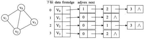

The graph above is an undirected graph with four vertices. Four vertices V0, V1, V2 and V3 are accessed by an array, which is described by the following structure definition. The element type of the array is VertexNode, one field info is used to store vertex information, and the other field first Edge points to the edge node associated with the vertex. For EdgeNode, the toAdjVex field of the edge node represents the array subscript of the other vertex node on the edge. The next field is only used to point to the other vertex node. All edge nodes linked through the next have the same starting vertex.
Note: When describing a graph with an adjacency table, the traversal order of the graph has been determined. For example, when traversing the adjacency table of the above graph from the vertex of V0, no matter the depth-first search (DFS) or breadth-first search (BFS), the V1 node will be found first. In fact, from the graph on the left, V1, V2 and V3 can be regarded as V1, V2 and V3. Next traversal node.

The adjacency table structure is defined as follows:

typedef struct EdgeNode
{
    int toAdjVex;                               // The index of vertex array which this edge points to.
    float weight;                               // The edge weight.
    struct EdgeNode *next;                      // The next edge, note that it only means the next edge also links to the vertex which this edge links to.
} EdgeNode;

typedef struct VertexNode
{
    VERTEX_DATA_TYPE info;                      // The vertex info,.
    struct EdgeNode* firstEdge;                 // The first edge which the vertex points to.
} VertexNode;

typedef struct
{
    VertexNode adjList[VERTEX_NUM];             // Adjacency list, which stores the all vertexes of the graph.
    int vertextNum;                             // The number of vertex.
    int edgeNum;                                // The number of edge.
} AdjListGraph;

• adjacency matrix

The adjacency matrix is suitable for dense graphs (the number of edges is large). Its abstract description is as follows:

The graph above is an undirected weightless graph. It only uses 0 and 1 to indicate whether two vertices are connected. Of course, the usual way is to replace 1 with the weight of the edge and 0 with a very large number (e.g. __) to indicate that the vertices are not connected.

The structure of adjacency matrix is defined as follows:

typedef struct
{
    int number;
    VERTEX_DATA_TYPE info;
} Vertex;

typedef struct
{
    float edges[VERTEX_NUM][VERTEX_NUM];        // The value of this two dimensional array is the weight of the edge.
    int vertextNum;                             // The number of vertex.
    int edgeNum;                                // The number of edge.
    Vertex vex[VERTEX_NUM];                     // To store vertex.
} MGraph;

algorithm

Depth First Search

A sentence is described as "a road to black", and its recursive and non-recursive code is as follows:

• recursion

void dfsRecursion(AdjListGraph* graph, int startVertexIndex, bool visit[])
{
    printf("%c ", (graph -> adjList[startVertexIndex]).info);
    visit[startVertexIndex] = true;
    EdgeNode* edgeIndex = (graph -> adjList[startVertexIndex]).firstEdge;
    while (edgeIndex != NULL)
    {
        if (visit[edgeIndex -> toAdjVex] == false)
            dfsRecursion(graph, edgeIndex -> toAdjVex, visit);
        edgeIndex = edgeIndex -> next;
    }
}

Hint: The recursive traversal of DFS is somewhat similar to the preamble traversal of binary tree.

• non-recursive

The stack, an additional data structure, was borrowed.

void dfsNonRecursion(AdjListGraph* graph, int startVertextIndex, bool visit[])
{
    linked_stack* stack = NULL;
    init_stack(&stack);

    // Visit the start vertex.
    printf("%c ", (graph -> adjList[startVertextIndex]).info);
    visit[startVertextIndex] = true;
    EdgeNode* edgeNode = (graph -> adjList[startVertextIndex]).firstEdge;
    if (edgeNode != NULL)
        push(stack, edgeNode);
    while (!isEmptyStack(stack))
    {
        edgeNode = ((EdgeNode*)pop(stack)) -> next;
        while (edgeNode != NULL && !visit[edgeNode -> toAdjVex])
        {
            printf("%c ", (graph -> adjList[edgeNode -> toAdjVex]).info);
            visit[edgeNode -> toAdjVex] = true;
            push(stack, edgeNode);
            edgeNode = (graph -> adjList[edgeNode -> toAdjVex]).firstEdge;
        }
    }
}

Breadth First Search

BFS is an algorithm of "looking out one circle after another", which is realized by means of "circular queue":

void bfs(AdjListGraph* graph, int startVertexIndex, bool visit[])
{
    // Loop queue initialization.
    LoopQueue loopQ;
    loopQ.front = 0;
    loopQ.rear = 0;
    LoopQueue* loopQueue = &loopQ;
    enqueue(loopQueue, &(graph -> adjList[startVertexIndex]));
    printf("%c ", (graph -> adjList[startVertexIndex]).info);
    visit[startVertexIndex] = true;
    while (!isEmpty(loopQueue))
    {
        VertexNode* vertexNode = dequeue(loopQueue);
        EdgeNode* edgeNode = vertexNode -> firstEdge;
        while(edgeNode != NULL)
        {
            if (visit[edgeNode -> toAdjVex] == false)
            {
                printf("%c ", (graph -> adjList[edgeNode -> toAdjVex]).info);
                visit[edgeNode -> toAdjVex] = true;
                enqueue(loopQueue, &(graph -> adjList[edgeNode -> toAdjVex]));
            }
            edgeNode = edgeNode -> next;
        }
    }
}

Tips:

1. BFS algorithm is similar to the hierarchical traversal of binary tree.
2. The last node of BFS traversal is the "farthest" node from the starting node.

Minimum Spanning Tree

Prim

• algorithm

  1. Select any vertex from the graph as the starting node of the spanning tree.
  2. From the nodes outside the spanning tree set (the set of all the vertices that have been added to the spanning tree), a point with the least cost from the spanning tree set is selected and added to the spanning tree set.
  3. Repeat step 2 until all vertices are added to the spanning tree set.
• Code

float prim(MGraph* graph, int startVertex)
{
    float totalCost = 0;
    float lowCost[VERTEX_NUM];              // The value of lowCost[i] represents the minimum distance from vertex i to current spanning tree.
    bool treeSet[VERTEX_NUM];               // The value of treeSet[i] represents whether the vertex i has been merged into the spanning tree.

    // Initialization
    for (int i = 0; i < (graph -> vertextNum); i++)
    {
        lowCost[i] = graph -> edges[startVertex][i];        // Init all cost from i to startVertex.
        treeSet[i] = false;                                 // No vertex is in the spanning tree set at first.
    }

    treeSet[startVertex] = true;                            // Merge the startVertex into the spanning tree set.
    printf("%c ", (graph -> vex[startVertex]).info);
    for (int i = 0; i < (graph -> vertextNum); i++)
    {
        int minCost = MAX_COST;                             // MAX_COST is a value greater than any other edge weight.
        int newVertex = startVertex;

        // Find the minimum cost vertex which is out of the spanning tree set.
        for (int j = 0; j < (graph -> vertextNum); j++)
        {
            if (!treeSet[j] && lowCost[j] < minCost)
            {
                minCost = lowCost[j];
                newVertex = j;
            }
        }
        treeSet[newVertex] = true;                          // Merge the new vertex into the spanning tree set.

        /*

            Some ops, for example you can print the vertex so you will get the sequence of node of minimum spanning tree.

        */
        if (newVertex != startVertex)
        {
            printf("%c ", (graph -> vex[newVertex]).info);
            totalCost += lowCost[newVertex];
        }


        // Judge whether the cost is change between the new spanning tree and the remaining vertex.
        for (int j = 0; j < (graph -> vertextNum); j++)
        {
            if (!treeSet[j] && lowCost[j] > graph -> edges[newVertex][j])
                lowCost[j] = graph -> edges[newVertex][j];  // Update the cost between the spanning tree and the vertex j.
        }
    }
    return totalCost;
}

Union Find Set

• introduce

It is very easy to judge whether several different elements belong to the same set, because of this characteristic, and the search is the Kruskal algorithm.( Kruskal's algorithm ) Important tools.
In this example, we use an array as the "set" of the collection tool. The subscript of the array represents the sequence number of the elements in the collection, and the value of the subscript represents the subscript of the parent node of the node in the array. This array is a large set, and there are many small sets in the large set. The division is based on whether these elements belong to the same root node. The value of the root node is negative, and the absolute value is the number of elements in the set. Therefore, by constantly searching for the parent node of two elements until the root node is found. Then, it judges whether the root nodes are equal to each other to determine whether the two elements belong to the same set (in the Kruskal algorithm, that is, to judge whether the newly added nodes will form rings).

• Code

int findRootInSet(int array[], int x)
{
    if (array[x] < 0)
    {
        // Find the root index.
        return x;
    }
    else
    {
        // Recursively find its parent until find the root,
        // then recursively update the children node so that they will point to the root.
        return array[x] = findRootInSet(array, array[x]);
    }
}

// For merging the one node into the other set.
bool unionSet(int array[], int node1, int node2)
{
    int root1 = findRootInSet(array, node1);
    int root2 = findRootInSet(array, node2);
    if (root1 == root2)
    {
        // It means they are in the same set
        return false;
    }

    // The value of array[root] is negative and the absolute value is its children numbers,
    // when merging two sets, we choose to merge the more children set into the less one.
    if (array[root1] > array[root2])
    {
        array[root1] += array[root2];
        array[root2] = root1;
    }
    else
    {
        array[root2] += array[root1];
        array[root1] = root2;
    }
    return true;
}

Note that the above unionSet method is used to merge sets, mostly as an auxiliary tool of the Kruskar algorithm. The successful implementation of this method shows that the selected two nodes and their set can form an acyclic connected component. Each successful execution of this method, the state of each set is updated (because there are new nodes). Join) for subsequent judgment.

Shortest Path Algorithms

Single Source Shortest Path Algorithms-Dijkstra Algorithm s

Dijstera algorithm is used to calculate the shortest distance from all the nodes in a graph to a particular node, because the implementation of Dijstera algorithm only calculates the shortest distance from a given "source node" to other nodes, so the algorithm is also a "single source shortest path algorithm".

• step

  1. Each node of the graph is divided into two sets, one is visited set and the other is unvisited set. In the initial stage of the algorithm, a given "source node" that needs to be computed is added to visited set.
  2. Select a node closest to the source node from the unvisited set and add it to the visited set.
  3. Take the newly added node as a springboard and recalculate the shortest distance between the node in the unvisited set and the source node (since the newly added node may shorten the distance between the source node and the node in the unvisited set, special attention should be paid).
  4. Repeat step 2 until all nodes have been added to visited set.
• Code

void dijkstra(MGraph* graph, int startVertexIndex)
{
    // For storing the minimum cost from the arbitrary node to the start vertex.
    float minCostToStart[VERTEX_NUM];

    // For marking whether the node is in the set.
    bool set[VERTEX_NUM];

    // Initialization
    for (int i = 0; i < VERTEX_NUM; i++)
    {
        minCostToStart[i] = graph -> edges[i][startVertexIndex];
        set[i] = false;
    }

    // Add the start vertex into the set.
    set[startVertexIndex] = true;
    int minNodeIndex = startVertexIndex;

    for (int count = 1; count < VERTEX_NUM; count++)
    {
        int minCost = MAX_COST;

        // Find the adjacent node which is nearest to the startVertexIndex.
        for (int i = 0; i < VERTEX_NUM; i++)
        {
            if (!set[i] && minCostToStart[i] < minCost)
            {
                minCost = minCostToStart[minNodeIndex];
                minNodeIndex = i;
            }
        }

        // Add the proper node into the set
        set[minNodeIndex] = true;

        // After the new node is added into the set, update the minimum cost of each node which is out of the set.
        for (int i = 0; i < VERTEX_NUM; i++)
        {
            if (!set[i] && (graph -> edges[i][minNodeIndex]) < MAX_COST)
            {
                // The new cost of each node to source = the cost of new added node to source + the cost of node i to new added node.
                float newCost = minCostToStart[minNodeIndex] + graph -> edges[i][minNodeIndex];

                if (newCost < minCostToStart[i])
                    minCostToStart[i] = newCost;
            }
        }
    }

    printf("The cost of %c to each node:\n", (graph -> vex[startVertexIndex]).info);
    for (int i = 0; i < VERTEX_NUM; i++)
    {
        if (i != startVertexIndex)
            printf("-----> %c : %f\n", (graph -> vex[i]).info, minCostToStart[i]);
    }
}

Tip: The Dijstro algorithm is very similar to the Plym algorithm, especially step 2. Dijstro algorithm always chooses the nearest node from unvisited set to join visited set, while Plim algorithm always chooses the nearest node from the spanning tree set to join the spanning tree.

Floyd Algorithm, a multi-source shortest path algorithm

Unlike the Djestera algorithm, calling Freud algorithm once can calculate the shortest distance between any two nodes. Of course, you can also calculate the shortest path from multiple sources by calling Djestera algorithm many times.

• step

  1. Initialize minCost[i][j]. minCost[i][j] denotes the distance from node i to J.
  2. Introduce the third node (springboard) K to see if the value of minCost[i][j] can be reduced through the node k, and if so, update the value of minCost[i][j].
  3. Repeat step 2 until all nodes have been treated as k.
• Code

void floyd(MGraph* graph)
{
    float minCost[VERTEX_NUM][VERTEX_NUM];          // Store the distance between any two nodes.
    int path[VERTEX_NUM][VERTEX_NUM];               // Store the intermediate node between the two nodes.
    int i, j, k;

    // Initialization
    for (i = 0; i < VERTEX_NUM; i++)
    {
        for (j = 0; j < VERTEX_NUM; j++)
        {
            minCost[i][j] = graph -> edges[i][j];
            path[i][j] = -1;
        }
    }

    // Find if there is another k node, it makes the distance dis[i][k] + dis[k][j] < dis[i][j];
    for (k = 0; k < VERTEX_NUM; k++)
        for (i = 0; i < VERTEX_NUM; i++)
            for (j = 0; j < VERTEX_NUM; j++)
            {
                if (minCost[i][j] > minCost[i][k] + minCost[k][j])
                {
                    minCost[i][j] = minCost[i][k] + minCost[k][j];
                    path[i][j] = k;
                }
            }

    for (i = 0; i < VERTEX_NUM; i++)
        for (j = 0; j < VERTEX_NUM; j++)
        {
            if (i != j && minCost[i][j] != MAX_COST)
                printf("%c ---> %c, the minimum cost is %f\n", (graph -> vex[i]).info, (graph -> vex[j]).info, minCost[i][j]);
        }
}