The second course of artificial intelligence - logical regression

Iris Iris The data set contains three categories: iris setosa, iris versicolor and iris virginica, with a total of 150 records, 50 data in each category, and each record has four characteristics: calyx length, calyx width, petal length and petal width.

Introduction to linear classifier

Linear classifier through feature linear combination To make classification decisions. For example, for a binary classification problem, it can be assumed that a linear classification is used Hyperplane Division of high-dimensional space: all points on one side of the hyperplane are classified as "yes", and the other side is classified as "no".

Main steps of designing linear classifier

1. Collect a group of samples with category marks X={x1,x2,..., xN}
2. Determine a criterion function J as needed, its value reflects the performance of the classifier, and its extreme value solution corresponds to the "best" decision
3. Use the optimization technology to find the extreme value solutions w * and w0 * of the criterion function J, so as to determine the discriminant function and complete the classifier design
4. Obtain the linear discriminant function g(x)=wT+w0 or g(x)=a*Ty. For the unknown sample x, calculate g(x) and judge its category

Use of logistic regression model in Sklearn

1. Import model:

from sklearn.linear_model import LogisticRegression

2. Fit training:

Note: call the fit(x, y) method to train the model, where x is the attribute of the data and Y is the type

clf = LogisticRegression()
print(clf)
clf.fit(train_feature,label)

3. Forecast:

predict['label'] = clf.predict(predict_feature)

Implementation of linear multi classification

-- because the length and width of petals and calyx of different species of iris are different, they are classified based on the length and width of petals and calyx

1. Use Jupiter notebook for linear classification

2. Multi classification linear coding

① Import iris dataset

iris=datasets.load_iris()
X=iris.data
print(X)
Y=iris.target
print(Y)

Note: iris has two attributes data，iris.target. Data is a matrix. Each column represents the length and width of sepals or petals. There are 4 columns in total. Each row represents a measured iris plant. A total of 150 records are sampled

Iris data are as follows:

[[5.1 3.5 1.4 0.2]
 [4.9 3.  1.4 0.2]
 [4.7 3.2 1.3 0.2]
 [4.6 3.1 1.5 0.2]
 [5.  3.6 1.4 0.2]
        ...
 [6.7 3.  5.2 2.3]
 [6.3 2.5 5.  1.9]
 [6.5 3.  5.2 2. ]
 [6.2 3.4 5.4 2.3]
 [5.9 3.  5.1 1.8]]

② Data processing

#Normalization processing
X = StandardScaler().fit_transform(X)
print(X)

Note: the specific function of normalization is to summarize the statistical distribution of unified samples. Normalization between 0-1 is the statistical probability distribution.

③ Training model

lr = LogisticRegression()   
lr.fit(X, Y)

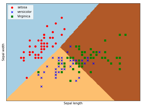
④ Draw image

import matplotlib.pyplot as plt
import numpy as np
from sklearn.datasets import load_iris   
from sklearn.linear_model import LogisticRegression 
 
#Load dataset
iris = load_iris()         
X = X = iris.data[:, :2]   #Get two column dataset
Y = iris.target           
 
#Logistic regression model
lr = LogisticRegression(C=1e5)  
lr.fit(X,Y)
 
#The meshgrid function generates two grid matrices
h = .02
x_min, x_max = X[:, 0].min() - .5, X[:, 0].max() + .5
y_min, y_max = X[:, 1].min() - .5, X[:, 1].max() + .5
xx, yy = np.meshgrid(np.arange(x_min, x_max, h), np.arange(y_min, y_max, h))
 
#The pcolormesh function draws the two grid matrices XX and YY and the corresponding prediction result Z on the picture
Z = lr.predict(np.c_[xx.ravel(), yy.ravel()])
Z = Z.reshape(xx.shape)
plt.figure(1, figsize=(8,6))
plt.pcolormesh(xx, yy, Z, cmap=plt.cm.Paired)
 
#Scatter plot
plt.scatter(X[:50,0], X[:50,1], color='red',marker='o', label='setosa')
plt.scatter(X[50:100,0], X[50:100,1], color='blue', marker='x', label='versicolor')
plt.scatter(X[100:,0], X[100:,1], color='green', marker='s', label='Virginica') 
 
plt.xlabel('Sepal length')
plt.ylabel('Sepal width')
plt.xlim(xx.min(), xx.max())
plt.ylim(yy.min(), yy.max())
plt.xticks(())
plt.yticks(())
plt.legend(loc=2) 
plt.show()

Examples of results:

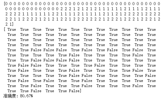
⑤ Accuracy test

y_hat = lr.predict(X)
Y = Y.reshape(-1)
result = y_hat == Y
print(y_hat)
print(result)
acc = np.mean(result)
print('Accuracy: %.2f%%' % (100 * acc))

Test results:

Topics: Python Algorithm AI logistic regressive

Programmer Think