Introduction: logistic regression is a very common means of classification. It belongs to probabilistic nonlinear regression, which is divided into two classification and multi classification regression models. For binary logistic regression, the dependent variable y has only two values of "yes" and "no", which are recorded as 1 and 0. Suppose that under the action of independent variables x1,x2,..., xp, the probability of y taking "yes" is p, and the probability of taking "no" is 1-p.

Logistic regression is a very common means of classification. It belongs to probabilistic nonlinear regression, which is divided into two classification and multi classification regression models. For binary logistic regression, the dependent variable y has only two values of "yes" and "no", which are recorded as 1 and 0. Suppose that under the action of independent variables x1,x2,..., xp, the probability of y taking "yes" is p, and the probability of taking "no" is 1-p. The following will introduce the principle and application of the most commonly used binary logistic regression model. (those who don't want to see the principle can be directly adjusted to the second half, with code demonstration)

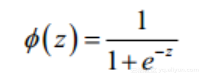
sigmoid function

In the binary classification problem of logistic regression, the function to be used is sigmoid function. Sigmoid function is very simple. Its expression is

The value range of dependent variable x is (- ∞, + ∞), but the value range of sigmoid function is (0,1). Therefore, no matter what value x takes, its corresponding sigmoid function value will fall into the range of (0,1). Its basic graphics are as follows:

 

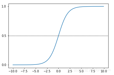
(when z is 0, the function value is 0.5; with the increase of z, the function value approaches 1; with the decrease of z, the function value approaches 0.)
Code for generating sigmoid function diagram:

import numpy
import math
import matplotlib.pyplot as plt

def sigmoid(x):
    a = []
    for item in x:
        a.append(1.0/(1.0 + math.exp(-item)))
    return a

x = numpy.arange(-10, 10, 0.1)
y = sigmoid(x)
plt.plot(x,y)
plt.yticks([0.0, 0.5, 1.0])
plt.axhline(y=0.5, ls='dotted', color='k')
plt.show()

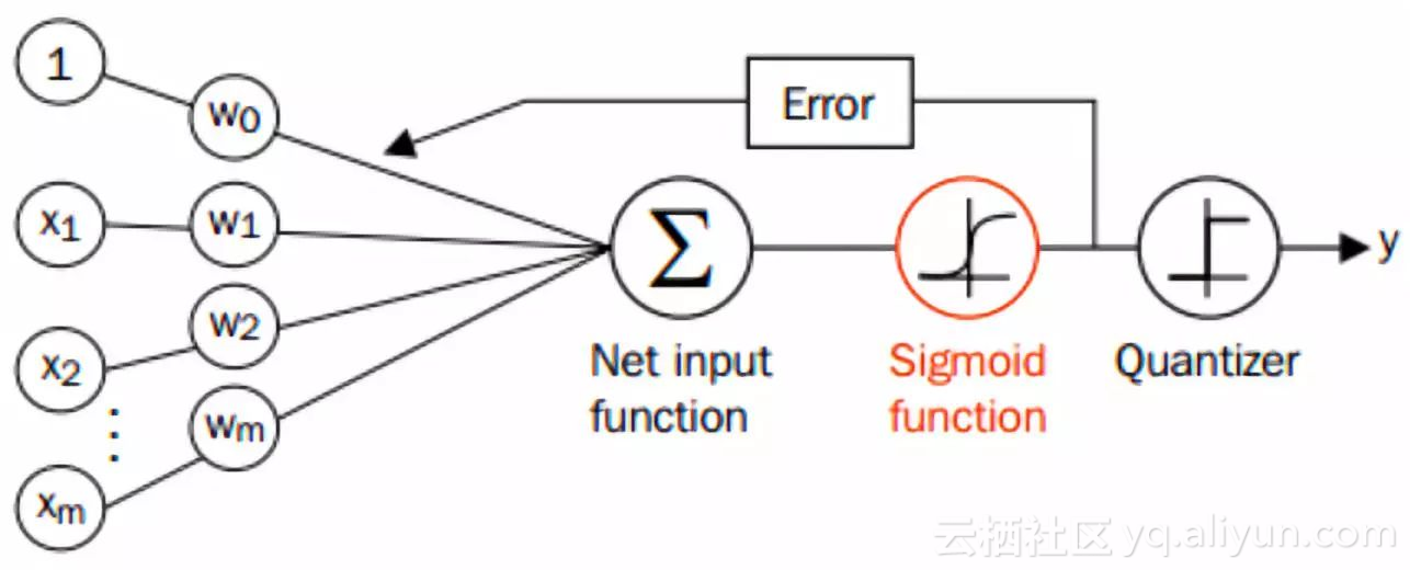
Sigmoid function is very suitable for the classification function of binary classification we just mentioned. Assuming that the characteristics of the input data are (x0, x1, X2,..., xn), we multiply each characteristic by a regression coefficient (W0, W1, W2,..., WN), and then accumulate to obtain the input z of the sigmoid function:

 

Then, the output is a value between 0 and 1. We classify the data whose output is greater than 0.5 into class 1 and the data whose output is less than 0.5 into Class 0. This is the classification process of Logistic regression.

Determination of optimal regression coefficient based on optimization method

From the above, we can see that the general process of logistic regression is as follows. What we need to do is to determine the best w = (W0, W1, W2,..., WN).

Loss function and maximum likelihood function

In logistic regression, the maximum likelihood method is used to solve the model parameters. For the concept of likelihood function, please refer to Kevin Gao's blog

http://www.cnblogs.com/kevinGaoblog/archive/2012/03/29/2424346.html

First define the likelihood function (each sample is considered to be independent):

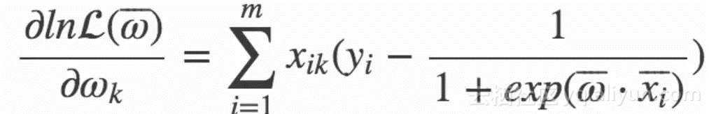
According to the concept of likelihood function, the probability that maximizes the likelihood function is the most reasonable. We want to maximize the likelihood function for ease of calculation, so we take logarithm

It can be seen that when the weight vector w maximizes l(w), W is the most reasonable.

Calculation of parameters by gradient rising method

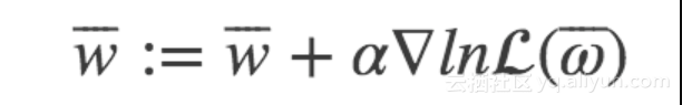
The basic idea of gradient rising method is: to find the maximum value of a function, the best way is to search along the gradient direction of the function. If the function is f, the gradient is recorded as D, and a is the step size, the iterative formula of the gradient rise method is: w: w+a*Dwf(w). The condition for stopping the formula is that the number of iterations reaches a specified value or the algorithm reaches an allowable error range. First, calculate the gradient of logarithmic function:

Directly expressed as a gradient by matrix multiplication:

Set the step size to α, Then the new weight parameters obtained by iteration are:

In this way, the process of Logistic regression through maximum likelihood estimation by gradient rise method is very clear. For the rest, we need to realize Logistic regression through code.

code implementation

Data set: the gre, gpa and rank information of students are used as variables to predict whether to admit. If admit=1, admit=0 means not to admit.

import pandas as pd
import statsmodels.api as sm
import pylab as pl
import numpy as np

df = pd.read_csv("binary.csv")

# Browse datasets
print (df.head())
#   admit  gre   gpa  rank
#0      0  380  3.61     3
#1      1  660  3.67     3
#2      1  800  4.00     1
#3      1  640  3.19     4
#4      0  520  2.93     4

# Rename the 'rank' column because there is a method named 'rank' in the dataframe
df.columns = ["admit", "gre", "gpa", "prestige"]

#Data statistics
print (df.describe())
#            admit         gre         gpa   prestige
#count  400.000000  400.000000  400.000000  400.00000
#mean     0.317500  587.700000    3.389900    2.48500
#std      0.466087  115.516536    0.380567    0.94446
#min      0.000000  220.000000    2.260000    1.00000
#25%      0.000000  520.000000    3.130000    2.00000
#50%      0.000000  580.000000    3.395000    2.00000
#75%      1.000000  660.000000    3.670000    3.00000
#max      1.000000  800.000000    4.000000    4.00000

# Frequency table, indicating the quantitative relationship between prestige and admin values
print (pd.crosstab(df['admit'], df['prestige'], rownames=['admit']))
#prestige   1   2   3   4
#admit                   
#0         28  97  93  55
#1         33  54  28  12

Quasi variable (dummy variable)

Dummy variables, also known as dummy variables, can be used to represent the possible influence of classified variables and non quantitative factors. In econometric models, the influence of attribute factors needs to be often considered. For example, it is often difficult to directly measure the size of attribute factors such as occupation, education level and season. Only their "Yes-D=1" or "No-D=0" or their degree or grade can be given. In order to reflect attribute factors and improve the accuracy of the model, attribute factors must be "quantified". The attribute factors are quantified by constructing 0-1 artificial variables. pandas provides control over a range of categorical variables. We can use get_dummies to virtualize the "prestige" column.

# Set prestige as a dummy variable
dummy_ranks = pd.get_dummies(df['prestige'], prefix='prestige')
print (dummy_ranks.head())
#   prestige_1  prestige_2  prestige_3  prestige_4
#0           0           0           1           0
#1           0           0           1           0
#2           1           0           0           0
#3           0           0           0           1
#4           0           0           0           1

To build a data frame that requires logistic regression:

# In addition to admit, gre and gpa, the above common virtual variables are added (note that the number of columns of virtual variables introduced should be the total number of columns of virtual variables minus 1, and the subtracted column should be used as the benchmark)
cols_to_keep = ['admit', 'gre', 'gpa']
data = df[cols_to_keep].join(dummy_ranks.ix[:, 'prestige_2':])
print (data.head())
#  admit  gre   gpa  prestige_2  prestige_3  prestige_4
#0      0  380  3.61           0           1           0
#1      1  660  3.67           0           1           0
#2      1  800  4.00           0           0           0
#3      1  640  3.19           0           0           1
#4      0  520  2.93           0           0           1

# You need to add the intercept variable required by logistic regression
data['intercept'] = 1.0

Perform logistic regression according to the above data frame:

# Specify columns as training variables, excluding target columns ` admit`
train_cols = data[data.columns[1:]]
# sigmoid function
def sigmoid(inX):  #sigmoid function
    return 1.0/(1+np.exp(-inX))
#Gradient rise for optimal parameters
def gradAscent(dataMat, labelMat): 
    dataMatrix=np.mat(dataMat) #Convert the read data into a matrix
    classLabels=np.mat(labelMat).transpose() #Convert the read data into a matrix
    m,n = np.shape(dataMatrix)
    alpha = 0.00001  #Set the threshold value of the gradient. The larger the value, the greater the gradient rise
    maxCycles = 300 #The number of iterations is usually set according to the actual data. Some may be 200 times
    weights = np.ones((n,1)) #Set the initial parameters and assign the default value to 1. Note that the weight here represents three parameters in matrix form.
    for k in range(maxCycles):
       h = sigmoid(dataMatrix*weights)
       error = (classLabels - h)     #Difference after derivation
       weights = weights + alpha * dataMatrix.transpose()* error #Iterative update weight
    return weights

#Get weight
weights=gradAscent(train_cols, data['admit']).getA()
#print (weights)

According to the fitted model, it can be predicted:

# For convenience here, we will copy a copy of the training set as the prediction set (excluding the admin column)
import copy
test_data = copy.deepcopy(data)

# The intercept variable should also be added to the prediction set
test_data['intercept'] = 1.0

# The columns in the data should be consistent with those used in the prediction
predict_cols = test_data[test_data.columns[1:]] 

# Make a prediction and store the prediction score in the predict column
predict=[]
test=np.mat(predict_cols)
for i in test:
    sum=sigmoid(i*np.mat(weights))
    print (sum)
    if sum <= 0.5:
        predict.append('0')
    else:
        predict.append('1')
test_data['predict']=predict

#Calculate prediction accuracy
predict_right=0
for i in range(0,400):
    if int(test_data.loc[i,'admit'])==int(test_data.loc[i,'predict']):
        predict_right=1+predict_right
    else:
        predict_right=predict_right
print ("Prediction accuracy:")
print ("%.5f" %(predict_right/400)) 
#Prediction accuracy:
#0.68250

From the above, we can see that the accuracy of the model prediction is 68.25%, but we often improve the gradient rise method to improve the prediction accuracy, for example, change to the random gradient rise method. The idea of random gradient rise method is to use only one data sample point at a time to update the regression coefficient. This greatly reduces the computational overhead.

def stocGradAscent(dataMatrix,classLabels):
    m,n=shape(dataMatrix)
    alpha=0.01
    weights=ones(n)
    for i in range(m):
        h=sigmoid(sum(dataMatrix[i] * weights))#numerical calculation
        error = classLabels[i]-h
        weights=weights + alpha * error * dataMatrix[i] #array and list matrix multiplication are different
    return weights

At the same time, the random gradient rise method can be improved as follows:

def stocGradAscent1(dataMatrix,classLabels,numIter=150):
    m,n=shape(dataMatrix)
    weights=ones(n)
    for j in range(numIter):
        dataIndex=list(range(m))
        for i in range(m):
            alpha=4/(1+i+j)+0.01#Ensure that the new data still has a certain influence after multiple iterations
            randIndex=int(random.uniform(0,len(dataIndex)))#Reduce cyclical fluctuations
            h=sigmoid(sum(dataMatrix[randIndex] * weights))
            error=classLabels[randIndex]-h
            weights=weights + alpha*dataMatrix[randIndex]*error
            del(dataIndex[randIndex])
    return weights

epilogue
From the above, you must have a certain understanding of logistic regression. If you don't want to define the function adjustment parameters yourself, you can also call the existing package for logistic regression classification, such as LogisticRegression in sklearn library and Logit in statsmodels library.

The original text was released on July 26, 2018
Author: carrot sauce
This article is from yunqi community partners“ Python enthusiast community ”, you can pay attention to relevant information“ Python enthusiast community"