Tianchi competition -- visual analysis of user emotion
catalogue
Tianchi competition -- visual analysis of user emotion
1, Read the data, check the basic situation and preprocess the data
Read data, basic analysis data
Null value processing, data mapping
Word segmentation analysis of comments
preface
This is a teaching competition in Tianchi Lake. It is not difficult as a whole. It is mainly an exercise in the basic data analysis of pandas.
The main contents of the topic are as follows
- Word cloud visualization (keywords in comments, word clouds with different emotions)
- Histogram (different topics, different emotions, different emotional words)
- Correlation coefficient heat map (different topics, different emotions, different emotional words)
The main data sources are as follows:
| Field name | type | describe | explain |
|---|---|---|---|
| content_id | Int | Data ID | / |
| content | String | Text content | / |
| subject | String | theme | Topics extracted or summarized according to context |
| sentiment_value | Int | Emotional analysis | Analyzed emotions |
| sentiment_word | String | Emotional words | Emotional words |
Let's directly analyze the data and complete the content
1, Read the data, check the basic situation and preprocess the data
When we get a data, we should check what information the data contains, whether there are default values in the data, and what values some column values have
Import related Library
import numpy as np
import pandas as pd
from pylab import *
import matplotlib.pyplot as plt
import seaborn as sns
import jieba
Read data, basic analysis data
#Read data
df = pd.read_csv('./data/earphone_sentiment.csv')
#View the first few lines of data
df.head()
#View basic data information
print(df.info())
print("----------------")
#View data missing information
print(df.isnull().sum())
print("----------------")
print(df['sentiment_word'].unique())
print("----------------")
print(df['sentiment_value'].value_counts())
The output is as follows. Here we mainly analyze the default values and {sentiments in the table_ The value of word column is because our analysis here is mainly aimed at emotional words (this competition is relatively simple, and emotional words are given directly)
<class 'pandas.core.frame.DataFrame'>
RangeIndex: 17176 entries, 0 to 17175
Data columns (total 5 columns):
 #   Column           Non-Null Count  Dtype
---  ------           --------------  -----
 0   content_id       17176 non-null  int64
 1   content          17176 non-null  object
 2   subject          17176 non-null  object
 3   sentiment_word   4966 non-null   object
 4   sentiment_value  17176 non-null  int64
dtypes: int64(2), object(3)
memory usage: 671.1+ KB
None
----------------
content_id             0
content                0
subject                0
sentiment_word     twelve thousand two hundred and ten
sentiment_value        0
dtype: int64
----------------
dtype: int64
 0    1 twenty-two ten
 1     4376
-1      590
Name: sentiment_value, dtype: int64
----------------
No evaluation    twelve twenty-one 0
 good       three thousand three hundred and two
 not bad       five hundred and sixty-nine
 difference        four hundred and fifteen
 strong        two hundred and forty-four
 cattle        one hundred and thirty-three
 garbage        thirty-two
 senior        thirty-one
 pursuit        twenty-six
 ha-ha        twenty-four
 Ugly        22
 fool         21
 noise        sixteen
 care        sixteen
 comfortable        16
 they hurt         fourteen
 Yin ran        14
 standard        12
 Boom         ten
 delicate         7
 Amazing         7
 conscience         7
 Speechless         6
 but         5
 uncomfortable        4
 Small         3
 adequate         3
 be fooled         2
 Spicy chicken         2
 vague         2
 turbidity         1
Name: sentiment_word, dtype: int64
Null value processing, data mapping
From the output data, we can analyze it according to sentiment_ The value pair of value is sentiment_word is divided into three categories: 0 for no evaluation, we regard it as neutral evaluation, 1 for high praise, and - 1 for poor evaluation. So do the following data preprocessing again - fill in the upper value and correct the sentiment_value mapping
# Fill in the sky value
df['sentiment_word'].fillna('No evaluation', inplace=True)
# Set sentiment_value mapping
map_sentiment_value = {-1: 'negative comment', 0: 'Middle evaluation', 1: 'Praise'}
df['sentiment_value'] = df['sentiment_value'].map(map_sentiment_value)
Make a perspective between emotional words and themes, and you can intuitively see the situation of praise, bad comment and medium comment in each theme
# Do sentiment_value PivotTable
df_pivot_table = df.pivot_table(index='subject', columns='sentiment_value', values='sentiment_word',
                                aggfunc=np.count_nonzero)

df_r_pivot_tabel = df.pivot_table(index='sentiment_value', columns='subject', values='sentiment_word',
                                   aggfunc=np.count_nonzero)
sentiment_value Middle evaluation Positive and negative comments subject Price 495 256 42 other 9493 2837 326 function 83 63 10 appearance 85 sixty-eight 5 comfortable 10 37 22 to configure 1452 759 121 tone quality 592 356 64 subject Price Other functions, comfortable appearance Configure sound quality sentiment_value Middle evaluation 495 9493 83 85 10 1452 592 Praise 256 2837 63 68 37 759 356 negative comment 42 326 10 5 22 121 64
Word segmentation analysis of comments
We also need to analyze the content comment part of the data, and there are many unnecessary contents in the comments. We need to segment this word and remove the stop words (i.e. some connectives to help us analyze). For comment segmentation, we mainly use the jieba word segmentation package. Stop words are commonly used Chinese stop words. You can get it at the link below.
Chinese common stop words list
stopwords = []
with open('./data/mStopwords.txt', encoding='utf-8') as f:
    for line in f:
        stopwords.append(line.strip('\n').split()[0])

# segment text by words
rows, cols = df.shape
cutwords = []
for i in range(rows):
    content = df['content'][i]
    g_cutword = jieba.cut_for_search(content)
    cutword = [x for x in g_cutword if (len(x) > 1) and x not in stopwords]
    cutwords.append(cutword)

s1 = pd.Series(cutwords)
df['cutwords'] = s1
print(s1.value_counts())
With jieba, it's easy to get word segmentation done. The results are as follows.
0                      [Silent, Angel, expect, presence, Mutual appreciation, fine, voice]
1        [HD650, 1k, distortion, Vocal tract, Left vocal tract, Vocal tract, Right , about, go beyond, official, ...
2                                [Da Yinke, 17, anniversary, data, good-looking, cheap]
3               [bose, beats, apple, Consumer, at all, know, Have curve, existence]
4                                                 [not bad, data]
                               ...
17171                        [3000, price, hd650, S7, better, Earphone]
17172                          [hd800, Burst skin, normal, Root line, such, worried]
17173     [welding, once, That's all, 820, Original line, brand new, 800s, Original line, 99, Box, Didn't move]
17174                                             [Hurry, Move]
17175           [sommer, reference resources, diy, Two meters, cost, 600, about, Sling, Original line]
Because we have to do different emotional analysis, we according to sentiment_value, the table is divided into three tables: poor evaluation, medium evaluation and high praise.
# Segmentation according to emotion
df_pos = df.loc[df['sentiment_value'] == 'Praise'].reset_index(drop=True)
df_neu = df.loc[df['sentiment_value'] == 'Middle evaluation'].reset_index(drop=True)
df_neg = df.loc[df['sentiment_value'] == 'negative comment'].reset_index(drop=True)
Here, the basic preprocessing is over, and you have an intuitive understanding of the data. Later, you can visualize the above results by some means.
2, Word cloud visualization
If I want to use word cloud visualization, I mainly use WordCloud, an open-source package. If this package is installed directly with pip, there may be problems, so I ran this part directly on Baidu's AIstudio.
This library is also relatively simple to use. You only need to set your own txt files and patterns and adjust a package.
The pictures inside are black and white pictures casually found on the Internet
pos_txt = '/'.join(np.concatenate(pos_df['cutwords']))
neg_txt = '/'.join(np.concatenate(neg_df['cutwords']))
neu_txt = '/'.join(np.concatenate(neu_df['cutwords']))
neu_mask = imread('./data/neu.png')
pos_mask = cv.imread('./data/pos.png')
neg_mask = cv.imread('./data/neg.png')
# Draw praise word cloud
pos_wc = WordCloud(font_path='./data/simhei.ttf',background_color='white',mask=pos_mask).generate(pos_txt)
neg_wc = WordCloud(font_path='./data/simhei.ttf',background_color='white',mask=neg_mask).generate(neg_txt)
neu_wc = WordCloud(font_path='./data/simhei.ttf',background_color='white',mask=neu_mask).generate(neu_txt)

plt.subplot(1,3,1)
plt.imshow(pos_wc)
plt.title("Postive wordcloud")
plt.axis('off')
plt.subplot(1,3,2)
plt.imshow(neu_wc)
plt.axis('off')
plt.title("Neutural wordcloud")
plt.subplot(1,3,3)
plt.imshow(neg_wc)
plt.title("Negative wordcloud")
plt.axis('off')
plt.show()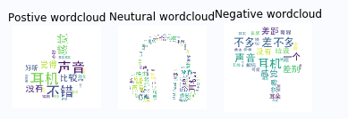
3, Histogram
The histogram mainly analyzes the number of comments under different topics and different emotional comments to see what users focus on.
# You can draw directly on the pivot table
df_pivot_table.plot.bar()
for x, y in enumerate(df_pivot_table['Middle evaluation'].values):
    plt.text(x - 0.2, y, str(y), horizontalalignment='right')
for x, y in enumerate(df_pivot_table['Praise'].values):
    plt.text(x, y, str(y), horizontalalignment='center')
for x, y in enumerate(df_pivot_table['negative comment'].values):
    plt.text(x + 0.2, y, str(y), horizontalalignment='left')
plt.title('Different topics, different emotional comments')
plt.ylabel('Number of comments')
plt.show()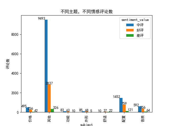
You can see that users mostly comment on price, configuration and sound quality, and more comments on other aspects.
Then we can see what more comments are saying in commendatory and derogatory words
# Take out the comment column in the commendatory and derogatory words
pos_word = df_pos['sentiment_word'].value_counts()
neg_word = df_neg['sentiment_word'].value_counts()
pos_word.plot.barh()
for x, y in enumerate(pos_word):
plt.text(y, x, str(y), horizontalalignment='left')
plt.xlabel('Number of comments')
plt.title('Statistics of commendatory words and comments')
plt.show()
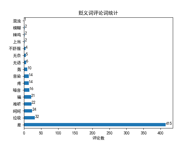
neg_word.plot.barh()
for x, y in enumerate(neg_word):
plt.text(y, x, str(y), horizontalalignment='left')
plt.xlabel('Number of comments')
plt.title('Statistics of derogatory words and comments')
plt.show()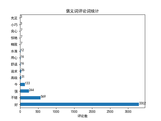
4, Thermodynamic diagram
The drawing of thermal diagram is mainly to see the correlation coefficients of different aspects of headphones. It mainly calls seaborn package, which is also very compatible with pandas.
# Thermodynamic diagram
sns.heatmap(df_r_pivot_tabel.corr(), annot=True)
plt.title('Thermodynamic diagram of correlation coefficient of different topics')
plt.show()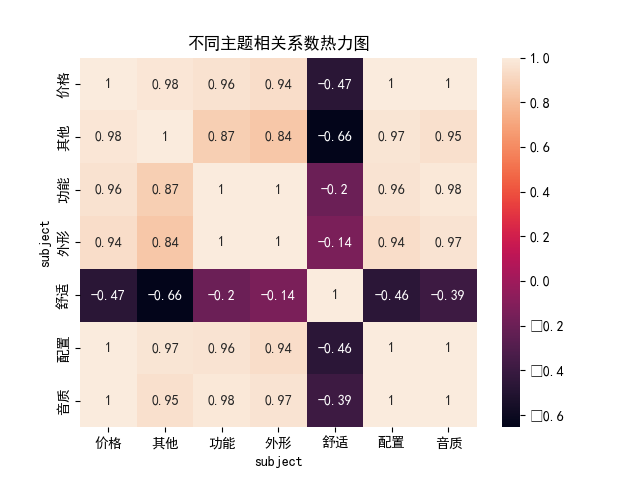
Obviously, comfort is negatively correlated with other aspects, while other functions are basically positively correlated.
summary
A very good game for learning pandas and some visualization.