I introduce

Anomaly detection (Anomaly detection) is one of the most mature applications of time series data analysis. It is defined as the process of identifying abnormal events or behaviors from normal time series. Effective anomaly detection is widely used in many real-world areas, such as quantitative transactions, network security testing, automatic driving vehicles and large-scale industrial equipment daily maintenance.

On this basis, we will present some of the previously mentioned deep / traditional machine learning algorithm models based on KDD99 and NSL_ The performance of KDD data set, combined with the specific data, the evaluation results of each model are given and summarized.

II KDD dataset

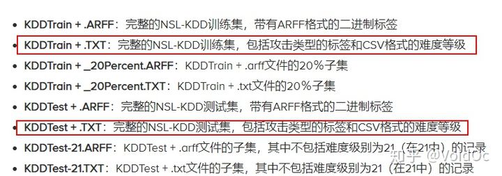
• KDDCup99

Introduction: https://blog.csdn.net/abrohambaby/article/details/78702512

Download link: KDD Cup 1999 Data

The complete set is very large, with about 500w data. It is recommended to use 10% of the data files with about 50w data to test the performance of the model.

• NSL_KDD

Introduction: https://www.unb.ca/cic/datasets/nsl.html

Download link: https://github.com/defcom17/NSL_KDD

NSL_KDD has made the following improvements on the basis of KDDCup99 data set:

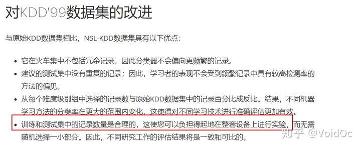
Generally, these two data sets are selected as Training data and Testing data:

III Data preprocessing

For continuous values, we use the MinMaxScaler provided by the scikit learn library to normalize the values

For discrete values, we use a one hot coding. encode_ The text function does this.

# Helper function for scaling continous values
def minmax_scale_values(training_df,testing_df, col_name):
    scaler = MinMaxScaler()
    scaler = scaler.fit(training_df[col_name].values.reshape(-1, 1))
    train_values_standardized = scaler.transform(training_df[col_name].values.reshape(-1, 1))
    training_df[col_name] = train_values_standardized
    test_values_standardized = scaler.transform(testing_df[col_name].values.reshape(-1, 1))
    testing_df[col_name] = test_values_standardized
    
    
#Helper function for one hot encoding
def encode_text(training_df,testing_df, name):
    training_set_dummies = pd.get_dummies(training_df[name]) # get_dummies is a way to realize one hot coding by using pandas
    testing_set_dummies = pd.get_dummies(testing_df[name]) 
    for x in training_set_dummies.columns:
        dummy_name = "{}_{}".format(name, x)
        training_df[dummy_name] = training_set_dummies[x]
        if x in testing_set_dummies.columns :
            testing_df[dummy_name]=testing_set_dummies[x]
        else :
            testing_df[dummy_name]=np.zeros(len(testing_df))
    training_df.drop(name, axis=1, inplace=True)
    testing_df.drop(name, axis=1, inplace=True)
    
    
sympolic_columns=["protocol_type","service","flag"]
label_column="Class"
for column in df.columns :
    if column in sympolic_columns:
        encode_text(training_df,testing_df, column)
    elif not column == label_column:
        minmax_scale_values(training_df,testing_df, column)

IV modeling

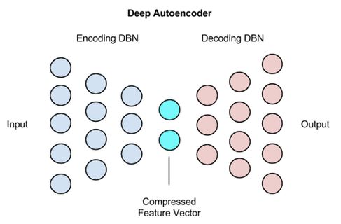
4.1 implementation of time series anomaly detection code based on AE self encoder (Tensorflow, Keras front-end interface)

• Model introduction

In order to avoid the imbalance of samples representing each attack type in the training data and avoid that the model cannot learn new attack types by observing the existing attack types, we propose a method to detect anomalies by using AE automatic encoder and reconstruction error.

In this method, we implement a sparse automatic encoder with input deletion, which is composed of 122 neuron input layers, because the number of features of each sample is 122, followed by the missing layer and the hidden layer of 8 neuron units Therefore, the hidden representation of the automatic encoder has a compression ratio of 122 / 8, forcing it to learn the relationship between interesting modes and features. Finally, there are 122 unit output layers, and the activation function of the hidden layer and the output layer is relu.

The automatic encoder is trained to reconstruct its input. In other words, it learns the identity function and trains the model only with the samples marked "normal" in the training data set, so as to capture the nature of normal behavior. This is through training the model to minimize the mean square error MSE (mean square error) between its output and input.

The regularization constraint imposed on the automatic encoder prevents it from simply copying the input to the output and over fitting the data. In addition, the lack of input makes the automatic encoder a special case of denoising automatic encoder. After training, this automatic encoder can reconstruct the input and delete it from the distorted damaged version, Force the automatic encoder to learn more data attributes.

About the details of the algorithm, I think Mr. Zhang's article is very good. You can expand and have a look.

Zhang Rong: time series anomaly detection algorithm based on self encoder 195 approval · 47 review article

• train

The Adam optimizer (batch size 100) was used to train the model for 10 epoch s. In addition, we retained 10% of the normal training samples as validation data to verify the effect of the model.

def getModel():
    input_layer = Input(shape=(x.shape[1],))
    encoded = Dense(8, activation='relu', activity_regularizer=regularizers.l2(10e-5))(input_layer) # l2 regularization constraint
    decoded = Dense(x.shape[1], activation='relu')(encoded)
    autoencoder = Model(input_layer, decoded)
    autoencoder.compile(optimizer='adam', loss='mean_squared_error')
    return autoencoder

autoencoder = getModel()
history = autoencoder.fit(
                            x[np.where(y0==0)],x[np.where(y0==0)],
                            epochs=10,
                            batch_size=100,
                            shuffle=True,
                            validation_split=0.1
                         )

Basically, the third epoch starts to converge, and the training speed is very fast, based on NSL_ For KDD, an epoch should be controlled within 15s.

• forecast

The model performs anomaly detection by calculating the reconstruction error of samples. Because the model is trained with normal data samples, the reconstruction error of samples representing attacks should be relatively high compared with the reconstruction error of normal data samples. This intuition enables us to detect attacks by setting a threshold for the reconstruction error, If the reconstruction error of the data sample is higher than the preset threshold, the sample is classified as attack, otherwise it is classified as normal traffic.

For the selection of threshold, two values can help guide the process, namely the Loss of training data set and verification data set. Through experiments, we found that the selection around these values will produce acceptable results. For our experiments, we set the Loss of model training data as the threshold.

Due to the nature of this method, it can only be used for class 2 classification, because it is only used for anomaly detection rather than classification.
Next, evaluate the performance of the test data set_ Losses is an auxiliary function, which accepts the original features and prediction features (the output of the automatic encoder) and returns the reconstruction loss of each data sample, and then reconstructs the error and preset threshold according to the classification of each data sample.

# calculate_losses is an auxiliary function to calculate the reconstruction loss of each data sample
def calculate_losses(x, preds):
    losses = np.zeros(len(x))
    for i in range(len(x)):
        losses[i] = ((preds[i] - x[i]) ** 2).mean(axis=None)
        
    return losses

# We set the threshold equal to the training loss of the automatic encoder
threshold = history.history["loss"][-1]

testing_set_predictions=autoencoder.predict(x_test)
test_losses=calculate_losses(x_test,testing_set_predictions)
testing_set_predictions=np.zeros(len(test_losses))
testing_set_predictions[np.where(test_losses>threshold)]=1

• assessment

To evaluate the model, we calculated the following performance indicators: Accuracy Recall Precision F1 Score

recall=recall_score(y0_test,testing_set_predictions)
precision=precision_score(y0_test,testing_set_predictions)
f1=f1_score(y0_test,testing_set_predictions)
print("Performance over the testing data set \n")
print("Accuracy : {} \nRecall : {} \nPrecision : {} \nF1 : {}\n".format(accuracy,recall,precision,f1 ))

• Summary

In this method, we try to overcome the problems existing in KDD99 and NSL-KDD data sets, that is, the class imbalance problem and the data are not consistent with the reality. By avoiding the attack data during training, we only use normal traffic to train the model, so it is not affected by the class imbalance of the data set. In addition, The fact that it only uses conventional traffic data for training makes it more valuable in real-world applications and more feasible in real networks.

Another advantage of this method is its simplicity. It is only composed of a single hidden layer of 8 neurons, so it is very easy to train, especially suitable for online learning. In the evaluation process, we avoid manual operation of the threshold to achieve reproducible results without manual interference. However, in the actual network, when deploying the system, the network administrator can manually adjust the threshold, so as to make a trade-off between sensitivity and specificity according to the network requirements. Compared with other existing methods, this is a huge advantage. In terms of detection rate, the performance of AE is also significant.

The obvious limitation of this method is that it can only distinguish between normal traffic and attack traffic (two classifiers rather than multiple classifiers), so it can not classify attacks into different attack types. This limitation can be overcome by establishing a set of models and other extended models. Its function can realize five-level classification.

• supplement

In addition, similar models include the improved model Dount based on VAE, which is linked as follows

https://github.com/NetManAIOps/donut​github.com/NetManAIOps/donut

Interested friends can have an in-depth understanding. On the whole, the effect of self encoder model in performing time series anomaly detection based on reconstruction error is very good. It is widely used in the industry (AIOps) and academia (peidan, Tsinghua).

4.2 based on LSTM_CNN's time series anomaly detection code implementation (Tensorflow, Keras front-end interface)

• Model introduction

CNN LSTM structure involves using convolutional neural network (CNN) layer for feature extraction in input data and combining LSTM to support sequence prediction. CNN LSTMs is developed for time series prediction problems (more widely used in NLP field) and application of image sequence to generate text description (e.g. video), but no one said that it could not be applied in KPIs time series anomaly detection scenario, right ~ so I also tried based on KDD dataset.

This architecture was originally called Long-term Recurrent Convolutional Network or LRCN model. Although we will use the more general name CNN LSTM to refer to CNN used in this lesson as the LSTM model in the previous paragraph. The key to this architecture is to use CNN model for feature extraction, and LSTM model helps the model learn features across time steps.

1.LSTM

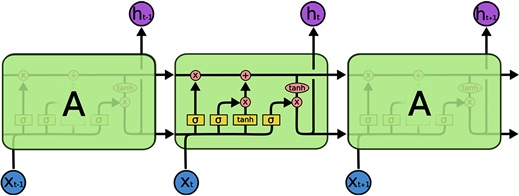
Long and short-term memory (LSTM) model is a special form of recurrent neural network (RNN), which can provide feedback at each neuron. The output of RNN depends not only on the input and weight of the current neuron, but also on the input of the previous neuron. Therefore, in theory, RNN structure is usually suitable for processing time series data. However, when dealing with a series of long-term related data samples, RNN will have the problems of gradient explosion and gradient disappearance, which has become the key point of introducing LSTM model later.

In order to overcome the gradient disappearance problem of RNN model, LSTM model includes an internal cycle of storing useful information and discarding useless information. There are four important elements in the flow chart of LSTM model: cell state, input gate, forgetting gate and output gate. The input, forget and output gates are used to update, maintain and delete the information contained in the control unit status. The forward calculation process can be expressed as:

Where Ct, Ct − 1 and C ˜ t represents the current cell state value, the cell state value at the previous time and the update of the current cell state value respectively. The symbols ft, it and ot represent forgetting gate, input gate and output gate respectively. Under appropriate parameter settings, according to equations (4) ~ (6), based on C ˜ The values of t and Ct calculate the output value ht. According to the difference between the output value and the actual value, all weight matrices are updated by back propagation through time (BPTT).

2.CNN

Convolutional neural network (CNN) may be the most commonly used deep learning neural network. At present, it is mainly used in image recognition / classification in the field of computer vision. For a large number of original data samples, CNN can usually effectively extract useful subsets of input data. Generally speaking, CNN is still a feedforward neural network, which is extended from multi-layer neural network (MLNN). The main difference between CNN and traditional MLNN is that CNN has the characteristics of sparse interaction and parameter sharing.

The traditional MLNN uses the full connection strategy to establish a neural network between the input layer and the output layer, which means that each output neuron has the opportunity to interact with each input neuron. Suppose there are m input neurons and n output neurons, and the weight matrix has M × n parameters. CNN by setting the size to k × The convolution kernel of k greatly reduces the parameters of the weight matrix. The two attributes of CNN improve the training efficiency of parameter optimization; Under the same computational complexity, CNN can train neural networks with more hidden layers, namely deep neural networks.

Temporal convolution neural network introduces a special one-dimensional convolution, which is suitable for processing univariate time series data. Temporal CNN doesn't use k × k convolution kernel, but use the size k × Convolution kernel of 1. After time convolution, the original univariate data set can be extended to m-dimensional feature data set. In this way, temporal CNN applies one-dimensional convolution to time series data, and expands univariate data set to multi-dimensional extracted features; The extended multidimensional feature data is more suitable for prediction using LSTM.

Therefore, we define a CNN LSTM model based on the Keras framework:

#import data
traindata = pd.read_csv('./data/kddtrain.csv', header=None)
testdata = pd.read_csv('./data/kddtest.csv', header=None)

X = traindata.iloc[:,1:42]
Y = traindata.iloc[:,0]
C = testdata.iloc[:,0]
T = testdata.iloc[:,1:42]

scaler = Normalizer().fit(X)
trainX = scaler.transform(X)

scaler = Normalizer().fit(T)
testT = scaler.transform(T)

y_train1 = np.array(Y)
y_test1 = np.array(C)

y_train= to_categorical(y_train1)
y_test= to_categorical(y_test1)


# reshape input to be [samples, time steps, features]
X_train = np.reshape(trainX, (trainX.shape[0],trainX.shape[1],1))
X_test = np.reshape(testT, (testT.shape[0],testT.shape[1],1))

Figure 1: low dimensional representation of samples in private network security data set: (1) each sample represents the network flow with 20 dimensions initially; (2) red / blue dots are abnormal / normal samples, (3) the horizontal axis represents the learned reduced one-dimensional space (4) the vertical axis represents the one-dimensional representation of reconstruction error caused by depth automatic coder.

• train

• # train the model
  # define parameters
  verbose, epochs, batch_size = 1, 10, 1000 
  n_timesteps, n_features, n_outputs = X_train.shape[1], X_train.shape[2],1 # 122,1,1
  
  # reshape output into [samples, timesteps, features]
  y_train = y_train.reshape((y_train.shape[0], 1, 1))
  
  # define model
  lstm_cnn = Sequential()
  lstm_cnn.add(Conv1D(filters=64, kernel_size=3, activation='relu', input_shape=(n_timesteps,n_features)))
  lstm_cnn.add(Conv1D(filters=64, kernel_size=3, activation='relu'))
  lstm_cnn.add(MaxPooling1D(pool_size=2))
  lstm_cnn.add(Flatten())
  lstm_cnn.add(RepeatVector(n_outputs))
  model.add(LSTM(200, activation='relu', return_sequences=True))
  lstm_cnn.add(Dropout(0.1))
  lstm_cnn.add(Dense(1, activation='sigmoid'))
  lstm_cnn.compile(loss="binary_crossentropy", optimizer="adam", metrics=['accuracy'])
  
  # set checkpoint
  checkpointer = callbacks.ModelCheckpoint(filepath="results/lstm_cnn_results/checkpoint-{epoch:02d}.hdf5", verbose=1, save_best_only=True, monitor='val_acc',mode='max')
  
  # set logger
  csv_logger = CSVLogger('results/lstm_cnn_results/cnntrainanalysis1.csv',separator=',', append=False)
  
  # fit network
  lstm_cnn.fit(
              X_train, y_train, 
              epochs=epochs, 
              batch_size=batch_size,
              verbose=verbose,
              validation_split=0.1,
              callbacks=[checkpointer,csv_logger])

  binary_crossentropy is a cross entropy loss function, which is generally used for loss calculation of two classifications: This is a loss function between probabilities. You will find that loss is 0 only when the predicted value is equal to y, otherwise loss is a positive number. Moreover, the greater the probability difference, the greater the loss. (if a negative number appears, X or Y is not normalized)

• y_pred = lstm_cnn.predict_classes(X_test)
  
  y_pred = y_pred[:,0]
  accuracy = accuracy_score(y_test,y_pred)
  recall = recall_score(y_test,y_pred, average="binary")
  precision = precision_score(y_test,y_pred, average="binary")
  f1 = f1_score(y_test,y_pred, average="binary")
  print("Performance over the testing data set \n")
  print("Accuracy : {} \nRecall : {} \nPrecision : {} \nF1 : {}\n".format(accuracy,recall,precision,f1 ))

• Summary

• The model is affected by the class imbalance of the data set, and the Recall score is lower than that of AE, indicating that many attack s are missed and not detected, and the indirect impact F1 = 2precisionrecall/(precision+recall) is not as good as that of AE model.

  Another disadvantage is that the network is relatively complex and the training time will be relatively long.

  But one advantage is that it can do multiple classifiers. If you want to achieve five-level classification, you can do it

• additional

• Application of LSTM-CNN in disease prediction: Disease Prediction Models Based on Hybrid Deep Learning Strategy

  Disease prediction model based on hybrid deep learning algorithm m.hanspub org/journal/paper/34067

  

  4.3 implementation of time series anomaly detection code based on DAGMM (Tensorflow)

  Reference paper: deep authoring Gaussian mixture model for unsupervised analog detection

  Paper link: https://openreview.net/pdf?id=BJJLHbb0-

• Model introduction

• In this paper, a deep automatic coding Gaussian mixture model (DAGMM) is proposed, which is a deep learning framework, which solves the above challenges in unsupervised anomaly detection from several aspects.

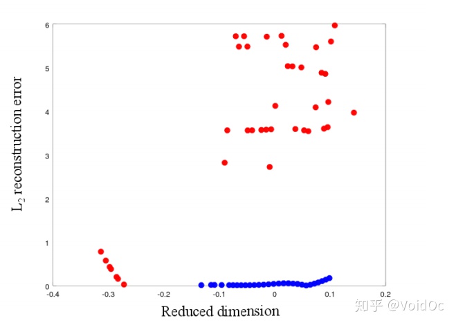
  Firstly, DAGMM retains the key information of input samples in a low dimensional space, which includes the characteristics of reduced dimensions found by dimension reduction and induced reconstruction error. From the example shown in Figure 1, we can see that the exception is different from the normal sample in two aspects:

  (1) Anomalies can deviate significantly in the reduced dimension, and their characteristics are related in different ways;

  (2) Compared with normal samples, anomalies are difficult to reconstruct. Only one aspect with suboptimal performance is involved (Zimek et al. (2012); Zhao et al (2016)), DAGMM performs dimensionality reduction through an automatic encoder using a sub network called a compression network, and prepares a low-dimensional representation for the input samples by connecting the reduced low-dimensional features from coding and the reconstruction error from decoding.

  

  secondly, DAGMM uses Gaussian mixture model (GMM) to process the density estimation task of Input data with complex structure in the learning low dimensional space, which is quite difficult for the simple model used in the existing work (Zhao et al (2016)). Although GMM has strong capabilities, it also introduces new challenges in model learning. Because GMM usually adopts such as expectation maximization (EM) (Huber) (2011)) and other alternating algorithms, so it is difficult to carry out the joint optimization of dimension reduction and density estimation. In order to make the GMM model learn better, GMM learning usually degenerates into the traditional two-step method: DAGMM uses a sub network called Estimation Network, which is from the compressed network (Compression Network) obtain the low dimensional Input of Input and output the "mixed member prediction" of each sample“ Using the membership of prediction samples, we can directly estimate the parameters of GMM to facilitate the evaluation of the energy / likelihood of Input samples. By minimizing the reconstruction error from the compressed network and the sample likelihood / energy from the estimated network at the same time.

• OVERVIEW

• The depth automatic coding Gaussian mixture model (DAGMM) consists of two main parts: compression network and estimation network. As shown in Figure 2, the working principle of DAGMM is as follows:

  

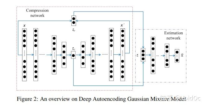
  (1) The compression network reduces the dimension of the input samples through the depth automatic encoder, prepares their low dimensional representation from the reduced space and reconstruction error characteristics, and provides the representation to the subsequent estimation network;

  (2) The estimation networks adopt feed and predict their likelihood (Energy) in the framework of Gaussian mixture model (GMM)

• train
• Fit Data to DAGMM Model
  next three points are different from original paper:
  
  - hiddens layers dimensions : [120,60,30,1] (original paper = [60,30,10,1])
  - 2 = 0.0001 (original paper = 0.005)
  - Add small value(10−6) to diagonal elements of GMM covariance (paper: no additional value)
  - Standard Scaler is applied to input data (This DAGMM implementation default)

• model = DAGMM(
                  comp_hiddens=[60, 30,10, 1], 
                  comp_activation=tf.nn.tanh,
                  est_hiddens=[10, 4], 
                  est_dropout_ratio=0.5, 
                  est_activation=tf.nn.tanh,
                  learning_rate=0.005, 
                  epoch_size=200,
                  minibatch_size=1024, 
                  random_seed=42
              )
  model.fit(X_train)

  The source code can refer to the Japanese https://github.com/tnakae/DAGMM/blob/master/KDDCup99.ipynb

• forecast

• Similarly, in this model, we judge the abnormal result based on the reconstruction error, and define the percentage of the predicted value less than or equal to a certain threshold in the total predicted number through the percentile function.

• y_pred = model.predict(X_test)
  
  # Energy thleshold to detect anomaly = 80% percentile of energies
  anomaly_energy_threshold = np.percentile(y_pred, 80) # Percentile function, at least 80% of data items are less than or equal to this value, and at least 20% of data items are greater than or equal to this value
  print(f"Energy thleshold to detect anomaly : {anomaly_energy_threshold:.3f}")
  
  # Detect anomalies from test data
  y_pred_flag = np.where(y_pred > anomaly_energy_threshold, 1, 0)

  prec, recall, fscore, _ = precision_recall_fscore_support(y_test, y_pred_flag, average="binary")
  print(f" Precision = {prec:.3f}")
  print(f" Recall    = {recall:.3f}")
  print(f" F1-Score  = {fscore:.3f}")

• Summary

• Finally, DAGMM is friendly to end-to-end training. Generally, it is difficult to learn deep automatic encoders through end-to-end training, because they are easy to fall into a less attractive local optimal state. Therefore, pre training is widely used in academia and industry to avoid this phenomenon. However, pre training limits the possibility of adjusting the dimensionality reduction behavior, because it is difficult to make any significant changes to the trained automatic encoder through fine tuning. Our empirical research shows that DAGMM is fully learned through end-to-end training, because the regularization introduced by the estimation network greatly helps the automatic encoder in the compression network get rid of the less attractive local optimal solution.

  Experiments on several common benchmark data sets show that DAGMM has superior performance over the existing technology, and the F1 score of anomaly detection is improved by 14%. In addition, we observe that the reconstruction error of the automatic encoder in DAGMM in end-to-end training is as low as that corresponding to its pre training, while the reconstruction error from the automatic encoder without regularization of the estimation network remains high. In addition, the end-to-end trained DAGMM is significantly superior to all baseline methods that rely on pre trained automatic encoders.

  

  Table 2: Average precision, recall, and F1 from DAGMM and the baseline methods. For each metric,the best result is shown in bold.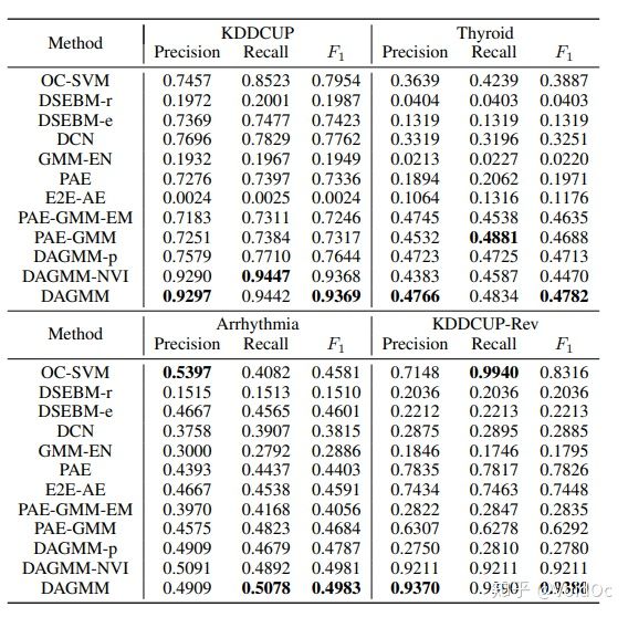

  4.4 implementation of time series anomaly detection code based on one class SVM

  Like AE and Isolation Forest, one class SVM can do single sample detection. The idea of this algorithm is very simple. It is to find a hyperplane and circle the positive examples in the sample. Prediction is to use this hyperplane for decision-making, and the samples in the circle are considered as positive samples. Because kernel function calculation is time-consuming, it is not used much in the scene of massive data;

• Model introduction

• One Class SVM also belongs to the support vector machine family, but it is different from the traditional classification regression support vector machine based on supervised learning. It is an unsupervised learning method, that is, it does not need us to mark the output label of the training set.

  So how can we find the divided hyperplane and support vector machine without class label? There are many solutions to the problem of One Class SVM. Here only a special idea SVDD is explained. For SVDD, we expect that all samples that are not abnormal are positive categories. At the same time, it uses a hypersphere rather than a hyperplane for division. The algorithm obtains the spherical boundary around the data in the feature space, hoping to minimize the volume of the hypersphere, so as to minimize the impact of abnormal point data.

  Assuming that the parameters of the generated hypersphere are the center o and the corresponding hypersphere radius r > 0, the hypersphere volume V(r) is minimized, and the center o is a linear combination of support lines; Similar to the traditional SVM method, the distance from all training data points xi to the center can be strictly less than R. But at the same time, a relaxation variable with penalty coefficient C is constructed ζ i. the optimization problem is shown in the figure below

  

  After the Lagrangian dual solution is adopted, it can be judged whether the new data point z is included. If the distance from z to the center is less than or equal to the radius r, it is not an abnormal point. If it is outside the hypersphere, it is an abnormal point.

  In Sklearn, we can use OneClassSVM in SVM package to detect outliers. OneClassSVM also supports kernel functions, so the parameter adjustment idea in ordinary SVM is also used here.

• train

• It should be noted that before modeling, the training error nu (within the range of (0,1]) needs to be set to represent the proportion of outliers; then, the kernel generally uses Gaussian kernel, which takes a lot of time to make psychological preparation.

• # we're using a one-class SVM, so we need.. a single class. the dataset 'label'
  # column contains multiple different categories of attacks, so to make use of 
  # this data in a one-class system we need to convert the attacks into
  # class 1 (normal) and class -1 (attack)
  
  data.loc[data['label'] == "normal.", "attack"] = 1  
  data.loc[data['label'] != "normal.", "attack"] = -1
  
  # grab out the attack value as the target for training and testing. since we're
  # only selecting a single column from the `data` dataframe, we'll just get a
  # series, not a new dataframe
  
  target = data['attack']
  
  # find the proportion of outliers we expect (aka where `attack == -1`). because 
  # target is a series, we just compare against itself rather than a column.
  
  outliers = target[target == -1]  
  print("outliers.shape", outliers.shape)  
  print("outlier fraction", outliers.shape[0]/target.shape[0])
  
  # drop label columns from the dataframe. we're doing this so we can do 
  # unsupervised training with unlabelled data. we've already copied the label
  # out into the target series so we can compare against it later.
  data.drop(["label", "attack"], axis=1, inplace=True)
  
  # check the shape for sanity checking.
  data.shape  
  
  from sklearn.model_selection import train_test_split  
  train_data, test_data, train_target, test_target = train_test_split(data, target, train_size = 0.8)  
  train_data.shape  
  
  from sklearn import svm
  
  # set nu (which should be the proportion of outliers in our dataset)
  nu = outliers.shape[0] / target.shape[0]  
  print("nu", nu)
  
  model = svm.OneClassSVM(nu=nu, kernel='rbf', gamma=0.00005)  
  model.fit(train_data) 

• Adjusting parameters
• assessment

• Some parameters can be introduced from https://www.cnblogs.com/wj-1314/p/10701708.html Let's find out. I won't talk about it here.

• preds = model.predict(test_data)  
  targs = test_target
  
  print("accuracy: ", metrics.accuracy_score(targs, preds))  
  print("precision: ", metrics.precision_score(targs, preds))  
  print("recall: ", metrics.recall_score(targs, preds))  
  print("f1: ", metrics.f1_score(targs, preds))  
  print("area under curve (auc): ", metrics.roc_auc_score(targs, preds)) 

• Summary
• Theoretically, it can only train one model for a time series, and different types of time series need to use different models. In this case, the cost of maintaining the model is relatively high, which is not suitable for large-scale time series anomaly detection scenarios;
• The effect of periodic curve is better. If it is burr data, it may not be applicable; Because long-term burr data can be regarded as normal data.
• Each parameter adjustment needs to set a certain threshold artificially or be defined according to the convergence value of training loss, which leads to the change of the threshold set in different time series (or after each training).

• 5 supplement

  5.1 reconstruction error threshold setting method

  This paper involves two methods to define the reconstruction error threshold, and I want to add it to you.

  a) Percentage threshold Percentile:

  P-Tile (i.e. p-quantile method) proposed by Doyle in 1962 is the oldest threshold selection method. In this method, the threshold is set according to the a priori probability, so that the proportion of target or background pixels after binarization is equal to the a priori probability. For example, in the training set, we know that the abnormality accounts for 80%, so the reconstruction error is sorted from small to large in the test set. The first 20% is normal and the last 80% is abnormal; For example, in the CV field, the proportion of known target or background pixels is equal to a priori probability; More simply, you already know the ratio of the target or background to the whole picture before finding the threshold.

  This method is simple and efficient, but it is powerless for data sets whose prior probability is difficult to estimate. Therefore, this method is not recommended for scenarios where the prior probability is unknown.

  b) Training the extremum after loss convergence

  The above introduces the basic principle of anomaly detection based on self encoder, which uses the large fluctuation (larger reconstruction error, greater than the threshold) of abnormal data in the process of encoding and decoding through automatic encoder to realize anomaly detection. So how to reasonably set the reconstruction error threshold to accurately detect anomalies?

  Since our training data only contains normal samples, one of the methods is to set the threshold value equal to the training loss of the automatic encoder, and then compare the reconstruction loss of each data sample in the test set with the threshold value. Those exceeding the threshold value are identified as abnormal.

  In addition, some experts in the CV field believe that setting a threshold on the L2 distance between the input image and the reconstructed image can effectively detect the attack image and so on.

  The selection of threshold has always been a metaphysical knowledge comparable to parameter adjustment. It is necessary to balance the false positive and false negative detection rates through multiple experiments or based on the so-called "expert experience", so as to optimize the detection effect of the model.

  6 summary there is a trade-off between false positive and false negative detection rates

  Generally speaking, in the time series anomaly detection scenario, the proportion of anomalies is very rare compared with the normal proportion. Therefore, in addition to supervised algorithms (classification and regression), anomaly detection algorithms based on unsupervised algorithms are also essential. In addition to Holt winters, ARIMA and other algorithms, some single sample two classifiers and models based on deep learning can also play a good detection effect.

  

  In particular, the self encoder model is outstanding in different data sets. We can use the reconstruction error and local error of the self encoder to achieve a good effect for the scene of anomaly detection of time series.

  This method can be used to provide some abnormal samples and increase the recall rate of abnormal detection. However, this method also has some disadvantages: