Today's brocade bag

Feature bag: time stamp and time series feature derivation of time series modeling

There are still many scenarios for the application of time series model in our daily work, such as predicting the future sales order quantity, predicting the stock price, predicting the trend of futures, predicting hotel occupancy, etc. This is also the reason why we must master time series modeling. The feature derivation of timestamp and time series value plays a great role in the modeling process! I wrote an article about date feature operation before—— "About date characteristics, you want to know that the operations are here ~" , you can first review the basic operation methods about date characteristics.

🚅 Index

01 introduction to time series data categories Derivation of 02 timestamp 03 derivative code sharing of timestamp 04 derivation of time series value 05 derivative code sharing of timing values

🏆 01 introduction to time series data categories

Let's take the classic time series model for example. Generally speaking, the data in the data set can be divided into three categories. 1) Y value: we also call it timing value. The sales volume field in the following table; 2) Time stamp: the field marking the occurrence time of this record, as shown in the statistical date field in the following table. oh, by the way, if it is not a single time series, such as the time series data of multiple stores recorded in the data set, it needs to be combined with the sequence attribute information, such as the store name and the city where the store is located; 3) Other fields: as the name suggests.

Today, we focus on the feature derivation of timestamp and timing value.

🏆 Derivation of 02 timestamp

Although the timestamp has only one field, it actually contains a lot of information. Generally speaking, we can disassemble it from the following angles and derive a series of variables. 1) Characteristics of timestamp itself Directly use Pandas series to extract timestamp features, such as which year, which quarter, which month, which week, which day, which time, which minute, which second, the day of the year, the day of the month, and the day of the week. 2) 0-1 features It is generally used in combination with real scenes, such as working days, weekends, public holidays (Spring Festival, Dragon Boat Festival, Mid Autumn Festival, etc.), X beginning, X middle, X End (X represents year, quarter, month and week), special festivals (such as operation suspension and service suspension), daily customary names (such as early morning, morning, noon, afternoon, evening, night, late night and early morning), Thus, the following can be derived:

• Is it a working day
• Spring Festival
• Is it at the beginning of the month
• Out of service
• Early morning
• Wait, wait

3) Time difference characteristics It is generally used in combination with real scenes, such as weekdays, weekends, etc., such as:

• N days before the Spring Festival
• N days before the weekend
• For example, there are still N days at the beginning of next month
• Wait, wait

🏆 03 derivative code sharing of timestamp

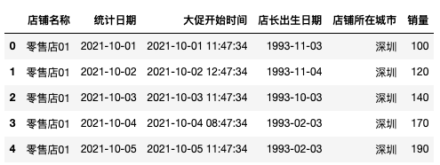
First, we fabricate some data to test the code.

# Import related library packages
import pandas as pd
import numpy as np
import datetime
import time
import random
from calendar import monthrange 

# Fabricated data
df = pd.DataFrame(
      [['Retail store 01', '2021-10-01', '2021-10-01 11:47:34', '1993-11-03', 'Shenzhen', 100],
       ['Retail store 01', '2021-10-02', '2021-10-02 12:47:34', '1993-11-04', 'Shenzhen', 120],
       ['Retail store 01', '2021-10-03', '2021-10-03 11:47:34', '1993-10-03', 'Shenzhen', 140],
       ['Retail store 01', '2021-10-04', '2021-10-04 08:47:34', '1993-02-03', 'Shenzhen', 170],
       ['Retail store 01', '2021-10-05', '2021-10-05 11:47:34', '1993-02-03', 'Shenzhen', 190],
       ['Retail store 01', '2021-10-06', '2021-10-06 15:47:34', '1993-04-03', 'Shenzhen', 10],
       ['Retail store 01', '2021-10-07', '2021-10-07 17:47:34', '1993-02-03', 'Shenzhen', 20],
       ['Retail store 01', '2021-10-08', '2021-10-08 19:47:34', '1993-06-03', 'Shenzhen', 420],
       ['Retail store 01', '2021-10-09', '2021-10-09 11:47:34', '1993-03-03', 'Shenzhen', 230],
       ['Retail store 01', '2021-10-10', '2021-10-10 20:47:34', '1993-02-20', 'Shenzhen', 80]
      ]
      ,columns=['Shop name', 'Statistical date', 'Start time of promotion', 'Store Manager date of birth', 'Store City', 'sales volume'])
df.head()

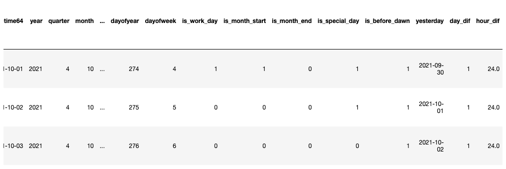
1) Characteristics of timestamp itself This is to extract the entity features of datetime itself, and use the Series method of Pandas.

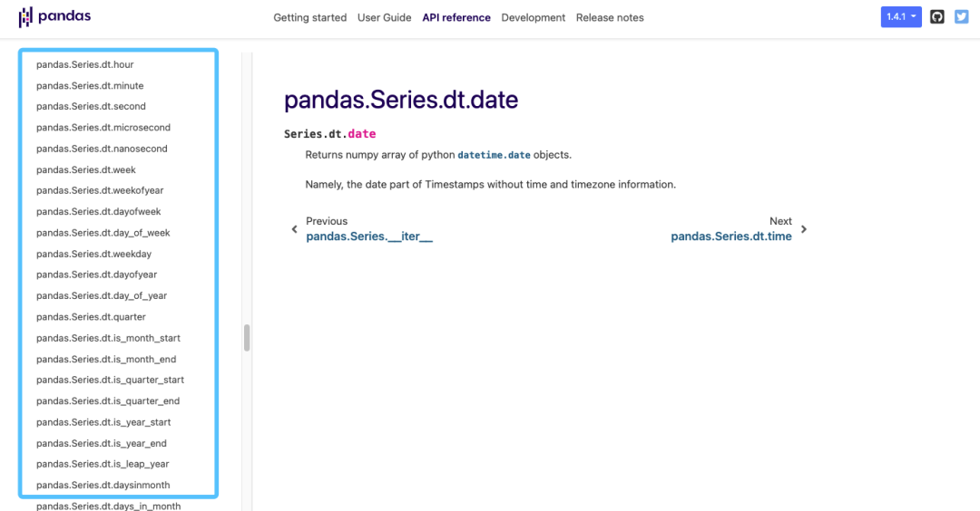
# It was originally a string and was converted to datetime
df['datetime64'] = pd.to_datetime(df['Statistical date'])
df['year'] = df['datetime64'].dt.year
df['quarter'] = df['datetime64'].dt.quarter
df['month'] = df['datetime64'].dt.month
df['week'] = df['datetime64'].dt.week
df['day'] = df['datetime64'].dt.day
df['hour'] = df['datetime64'].dt.hour
df['minute'] = df['datetime64'].dt.minute
df['second'] = df['datetime64'].dt.second
df['weekday'] = df['datetime64'].dt.weekday
df['weekofyear'] = df['datetime64'].dt.weekofyear
df['dayofyear'] = df['datetime64'].dt.dayofyear
df['dayofweek'] = df['datetime64'].dt.dayofweek

2) 0-1 features Here we need to introduce some dates about the real scene to judge whether it is true or not.

df['is_work_day'] = np.where(df['dayofweek'].isin([5,6]), 0, 1) # Is it a working day
df['is_month_start'] = np.where(df['datetime64'].dt.is_month_start, 1, 0)
df['is_month_end'] = np.where(df['datetime64'].dt.is_month_end, 1, 0)

# Special days / public holidays
special_day = ['2021-10-01','2021-10-02']
df['is_special_day'] = np.where(df['Statistical date'].isin(special_day), 1, 0)

# Early morning
df['is_before_dawn'] = np.where(df['hour'].isin([0,1,2,3]), 1, 0)

3) Time difference characteristics

# Get previous day's date
df['yesterday'] = df['datetime64'] - datetime.timedelta(days=1)
# Date difference calculation (days)
df['day_dif'] = (df['datetime64'] - df['yesterday']).dt.days
# Date difference calculation (hours)
df['hour_dif'] = (df['datetime64'] - df['yesterday']).values/np.timedelta64(1, 'h') # D is days

🏆 04 derivation of time series value

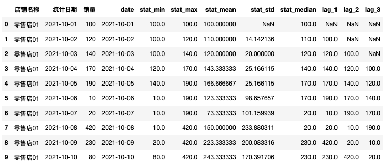
The time series value in this example is the sales volume field. Generally, we need to sort and complete the time series of the data before starting the operation. There are several angles for the characteristic derivation of the time series value. 1) Time sliding window statistics Based on the statistical data of a certain period of time window, also known as Rolling Window Statistics, the statistical methods generally include min/max/mean/median/std/sum, etc. for example, if we choose the sliding window as 7 days, the variables that can be derived are: the minimum / maximum / mean / median / variance / sum of sales in the past 7 days. When using such features, we should pay attention to the problem of multi-step prediction.

2) lag value lag can be understood as forward sliding time. For example, lag1 represents forward sliding for 1 day, that is, take the time series value of T-1 as the variable of the current time series.

🏆 05 derivative code sharing of timing values

1) Time sliding window statistics Because the method is called Rolling Window Statistics, there is also a method called rolling in the code for the implementation of this part. This method is very easy to use in timing modeling, which will be described in a separate article later.

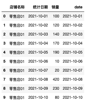
df = df.loc[:,['Shop name', 'Statistical date','sales volume']]
df['date'] = pd.to_datetime(df['Statistical date'])

# Remember to sort before deriving time series value features
df.sort_values(['Shop name', 'Statistical date'], ascending=[True,True], inplace=True)

# Derived time sliding window statistical variable
f_min = lambda x: x.rolling(window=3, min_periods=1).min()
f_max = lambda x: x.rolling(window=3, min_periods=1).max()
f_mean = lambda x: x.rolling(window=3, min_periods=1).mean()
f_std = lambda x: x.rolling(window=3, min_periods=1).std()
f_median=lambda x: x.rolling(window=3, min_periods=1).median()
function_list = [f_min, f_max, f_mean, f_std,f_median]
function_name = ['min', 'max', 'mean', 'std','median']
for i in range(len(function_list)):
    df[('stat_%s' % function_name[i])] = df.sort_values('Statistical date', ascending=True).groupby(['Shop name'])['sales volume'].apply(function_list[i])

2) lag value

# Derived lag variable
for i in [1,2,3]:
    df["lag_{}".format(i)] = df['sales volume'].shift(i)

📚 Reference

[1] Once made me doubt the time stamp feature processing skills of life. https://mp.weixin.qq.com/s/dUdGhWY8l77f1TiPsnjMQA [2] Time series tree model feature engineering summary https://blog.csdn.net/fitzgerald0/article/details/104029842 [3] Summary of multi-step prediction methods of time series https://zhuanlan.zhihu.com/p/390093091 [4] Characteristic engineering summary of time series data https://zhuanlan.zhihu.com/p/388551117 [5] Pandas Series dt https://pandas.pydata.org/docs/reference/api/pandas.Series.dt.date.html