Introduction: SQL optimization is the most important part of database performance optimization. The key of SQL optimization is inseparable from three points: table connection mode, access path and execution order. This paper focuses on several common connection modes.
For multi table Association query, the execution steps of the query optimizer are as follows.
1) Access path: multiple objects are involved in the query statement. The retrieval method of each object data can be determined based on the cost, whether to select full table scanning or index access, etc.
2) Connection method: the association method between result sets, mainly including nested loop, hash connection, sort merge connection, etc. The optimizer's judgment on the connection mode between result sets is particularly important, because the judgment result will directly affect the execution efficiency of SQL.
3) Association order: when there are more than 2 associated objects, first select the result set obtained by associating the two objects, and then associate it with the third result set.
Let's focus on several common connection methods.
Nested loop connection
Figure 1 shows a schematic diagram of nested loop connection.
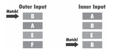 Figure 1 Schematic diagram of nested loop connection
The nested circular query process is as follows.
1) When the two tables are associated, the optimizer will first determine the driven table, also known as the outer table, and the other is the driven table, also known as the inner table. Generally, the optimizer will define a small amount of data as a driving table. In the execution plan, the driving table is above and the driven table is below.
2) After the drive table is confirmed, a row of valid data will be extracted from it, and the valid data will be found and matched in the driven table (internal table) and extracted.
3) Return the data to the client.
From the above steps, we can see that the number of rows returned by the driver table directly affects the access times of the driven table. For example, the driver table finally returns 10 rows of valid data according to the filter criteria. Each returned item will be passed to the driven table for matching. The driver table needs to be accessed circularly for 10 times. The example code is as follows:
SQL> SELECT /*+ USE_NL(e d) */ e.first_name, e.last_name, e.salary, d.department_name

  FROM hr.employees e, hr.departments d

 WHERE d.department_name IN ('Marketing', 'Sales')

   AND e.department_id = d.department_id;


SQL>  select * from table(dbms_xplan.DISPLAY_CURSOR(null, null, 'ALLSTATS LAST'));

SQL_ID  3nsqhdh150bx5, child number 0

-------------------------------------

SELECT /*+ USE_NL(e d) */ e.first_name, e.last_name, e.salary,

d.department_name   FROM hr.employees e, hr.departments d  WHERE

d.department_name IN ('Marketing', 'Sales')    AND e.department_id =

d.department_id


Plan hash value: 2968905875

-------------------------------------------------------------------------------------

| Id  | Operation          |Name       |Starts|E-Rows|A-Rows |   A-Time   | Buffers |

-------------------------------------------------------------------------------------

|   0 | SELECT STATEMENT   |           |    1 |      |    36 |00:00:00.01 |      23 |

|   1 |  NESTED LOOPS      |           |    1 |  19  |    36 |00:00:00.01 |      23 |

|*  2 |   TABLE ACCESS FULL|DEPARTMENTS|    1 |  2   |     2 |00:00:00.01 |      8 |

|*  3 |   TABLE ACCESS FULL|EMPLOYEES  |    2 |  10  |    36 |00:00:00.01 |     15 |

-------------------------------------------------------------------------------------
From the above example code, we can see that DEPARTMENTS is the driven table, Starts is 1, indicating that it is accessed only once and returns 2 rows of valid data (A-Rows is the actual number of rows returned), EMPLOYEES is the driven table, Starts is 2, indicating that it is accessed twice.
Students who have learned C + + programming should remember that nested loops in C + + are somewhat similar to the following loops:
#include <stdio.h>

int main ()

{

   int i, j;

   for(i=1; i<100; i++) {

      for(j=1; j <= 100; j++)

        if(!(i%j)) break;

      if(j > (i/j)) printf("%d \n", i);

   }

   return 0;

}
The number of cycles of J depends on the value range of i. We can regard i as the driven table and j as the driven table.
The performance of nested loop connection is mainly limited by the following points.
-
The number of rows returned by the drive table.
-
Access method of driven table: if the cardinality of the connected column of the driven table is small and the selectivity is poor, it will lead to the access method of full table scanning, and its efficiency will become very low. Therefore, we suggest that the connected column has an index with large cardinality and high selectivity.
-
A small amount of data will be returned after driving table filtering.
-
The associated field of the driven table needs to have an index (the cardinality of the join column is large or the selectivity is high).
-
After the two tables are associated, a small amount of data will be returned.
-
Suitable for OLTP system.
If the optimizer selects the wrong connection method, we can use hint to enforce the connection method using nested loops: "/ * + USE_NL(TABLE1,TABLE2) LEADING(TABLE1) * /, where TABLE1 and TABLE2 are aliases of associated tables, and LEADING(TABLE1) is used to specify TABLE1 as the driving table.
HASH join
Figure 2 shows a hash connection diagram.
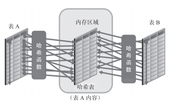 Figure 2 hash connection diagram
Nested loop connection is applicable to the case where a small amount of data will be returned after two tables are associated. What connection method should be used when a large amount of data is returned? The answer is to use hash connections.
The query process of hash connection is as follows.
1) The two tables are equivalently related.
2) The optimizer takes the table with small amount of data as the driving table, and constructs the connection column of the driving table into a hash table in the SQL work areas of PGA.
3) Read the large table and hash the connected columns (check the hash table to find the connected rows).
4) Return the data to the client.
From the above steps, we can see that matching by hash value is more suitable for the equivalent Association of two tables. The example code is as follows:
SQL> SELECT /*+ USE_HASH(o l) */o.customer_id, l.unit_price * l.quantity

  2    FROM oe.orders o, oe.order_items l

  3   WHERE l.order_id = o.order_id;


SQL> select * from table(dbms_xplan.DISPLAY_CURSOR(null, null, 'ALLSTATS LAST'));

SQL_ID  cu980xxpu0mmq, child number 0

-------------------------------------

SELECT /*+ USE_HASH(o l) */o.customer_id, l.unit_price * l.quantity

FROM oe.orders o, oe.order_items l  WHERE l.order_id = o.order_id


Plan hash value: 864676608

-------------------------------------------------------------------------------------------------------------

| Id  | Operation          |Name       |Starts|E-Rows|A-Rows|A-Time      |Buffers|Reads|OMem |1Mem |Used-Mem|

-------------------------------------------------------------------------------------------------------------

|   0 | SELECT STATEMENT   |           |   1  |      | 665  |00:00:00.04 |   57  |   5 |     |     |         |

|*  1 |  HASH JOIN         |           |   1  |  665 | 665  |00:00:00.04 |   57  |   5 |1888K|1888K|1531K (0)|

|   2 |   TABLE ACCESS FULL|ORDERS     |   1  |  105 | 105  |00:00:00.04 |   6   |   5 |     |     |         |

|   3 |   TABLE ACCESS FULL|ORDER_ITEMS|   1  |  665 | 665  |00:00:00.01 |   51  |   0 |     |     |         |

-------------------------------------------------------------------------------------------------------------
From the above example code, we can see that ORDERS is the drive table, Starts is 1, indicating that 105 rows of valid data are returned after one access (A-Rows is the actual number of rows returned), and ORDER_ITEMS is the driven table, and Starts is also 1, indicating that it is accessed only once. Among them, OMem and 1Mem are the PGA evaluation values required for execution, and used MEM is the memory consumed by the SQL working area in PGA during actual execution (i.e. the number of disk exchanges). When the drive table is large and the SQL working area of PGA cannot be fully accommodated, it will overflow into the temporary table space to generate disk interaction, which will affect the performance.
Hash connection performance is mainly limited by the following two points.
-
Equivalent connection.
-
When the PGA SQL workspace is small and the drive table is large, performance problems are easy to occur.
The hash join method is useful when both of the following conditions are met.
-
A large amount of data is returned after the two tables are equivalently associated.
- Unlike nested loop joins, hash joins do not require an index when connecting the join fields of the driven table.
Similarly, we can also use the prompt to enforce the use of hash connection: "/ * + USE_HASH (TABLE1,TABLE2) LEADING(TABLE1) * /".
Sort merge join
Figure 3 shows the sorting merge connection diagram.
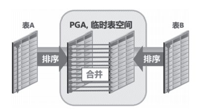 Figure 3} sorting and merging connection diagram
Hash connection is applicable to the case where two tables return a large amount of data after equivalent Association. What connection method should be used when non equivalent Association returns a large amount of data? The answer is sort merge join.
When the following conditions are met, the performance of sort merge connection is better than hash connection.
-
Non equivalent Association of two tables (>, > =, <, < =, < >).
-
The data source itself is orderly.
-
No additional sorting operations are necessary.
There is no concept of driving table in the sort merge connection method. The connection query process is as follows.
1) The two tables are sorted according to the associated columns.
2) Merge in memory.
From the above implementation steps, we can see that since the matching objects are the sorted values of the connected columns, the sorting merge connection method is more suitable for the case of non equivalent association between two tables. The example code is as follows:
SQL> SELECT o.customer_id, l.unit_price * l.quantity

  FROM oe.orders o, oe.order_items l

 WHERE l.order_id > o.order_id;

32233 rows selected..

SQL> select * from table(dbms_xplan.DISPLAY_CURSOR(null, null, 'ALLSTATS LAST'));

SQL_ID  ajyppymnhwfyf, child number 1

-------------------------------------

SELECT o.customer_id, l.unit_price * l.quantity   FROM oe.orders o,

oe.order_items l  WHERE l.order_id > o.order_id


Plan hash value: 2696431709

-----------------------------------------------------------------------------------------------------------

| Id  | Operation         |Name       |Starts| E-Rows | A-Rows | A-Time     |Buffers|OMem |1Mem | Used-Mem |

-----------------------------------------------------------------------------------------------------------

|   0 | SELECT STATEMENT  |           |    1 |        |  32233 |00:00:00.10 |  21   |     |     |          |

|   1 | MERGE JOIN        |           |    1 | 3 4580 |  32233 |00:00:00.10 |  21   |     |     |          |

|   2 | SORT JOIN         |           |    1 |    105 |    105 |00:00:00.01 |   4   |11264|11264|10240  (0)|

|   3 | TABLE ACCESS FULL |ORDERS     |    1 |    105 |    105 |00:00:00.01 |   4   |     |     |          |

|*  4 | SORT JOIN         |           |  105 |    665 |  32233 |00:00:00.05 |  17   |59392|59392|53248  (0)|

|   5 | TABLE ACCESS FULL |ORDER_ITEMS|    1 |    665 |    665 |00:00:00.01 |  17   |     |     |          |

------------------------------------------------------------------------------------------------------------
From the execution plan shown in the above example, we can see that the ORDERS table Starts with ID=3 is 1, which indicates that 105 rows of valid data are returned after one access (A-Rows is the actual number of returned rows), and order_ The Starts of the items table is 1, indicating that it is accessed only once, but the Starts of the SORT JOIN table with ID=4 is 105, indicating that 105 matches have been made in memory. Where, OMem and 1Mem are the PGA evaluation values required for sorting operation, and used MEM is the memory consumed by the SQL working area in PGA during actual execution (i.e. the number of disk exchanges).
From the above steps, we can see that the comparison object is the connected column order of the two tables_ ID, so the respective connection columns need to be sorted first (ID=2 and ID=4), and then matched. If there is an index on the connected column at this time, the data returned by the index is ordered, and no additional sorting operation is required at this time.
Similarly, we can also use the prompt to force the selection of sorting merge connection: "/ * + USE_MERGE(TABLE1,TABLE2) * /".
Cartesian connection
When one or more table connections do not have any connection conditions, the database will use Cartesian connections. The optimizer concatenates each row of one data source with each row of another data source to create a Cartesian product of two sets of data sets. The example code is as follows:
SQL> SELECT o.customer_id, l.unit_price * l.quantity

  FROM oe.orders o, oe.order_items l;

69825 rows selected.


SQL> select * from table(dbms_xplan.DISPLAY_CURSOR(null, null, 'ALLSTATS LAST'));

SQL_ID  d3xygy88uqzny, child number 0

-------------------------------------

SELECT o.customer_id, l.unit_price * l.quantity   FROM oe.orders o,

oe.order_items l

Plan hash value: 2616129901

-----------------------------------------------------------------------------------------------

| Id  | Operation            | Name      |Starts | E-Rows | Buffers |  OMem |  1Mem | Used-Mem |

-----------------------------------------------------------------------------------------------

|   0 | SELECT STATEMENT     |           |     1 |        |     125 |       |       |          |

|   1 |  MERGE JOIN CARTESIAN|           |     1 |  69825 |     125 |       |       |          |

|   2 |   TABLE ACCESS FULL  |ORDERS     |     1 |    105 |     108 |       |       |          |

|   3 |   BUFFER SORT        |           |   105 |    665 |      17 | 27648 | 27648 |24576  (0)|

|   4 |    TABLE ACCESS FULL |ORDER_ITEMS|     1 |    665 |      17 |       |       |          |

-----------------------------------------------------------------------------------------------
From the above implementation plan, we can see that we first set the table order_items, and then the Cartesian product of the two tables. Since there is no filter condition, when the amount of data is large, the number of returned rows will be very large. Therefore, it is not recommended to use a query without any connection condition unless there are special circumstances.
This article is excerpted from the DBA Breakthrough Guide: left hand Oracle, right hand MySQL.
This book is the painstaking work of senior Oracle and MySQL technical experts of meichuang technology. It accumulates the author's many years of experience and practical experience. It is also one of the few database technology books combining Oracle and MySQL in the market.
The book is mainly divided into Oracle and MySQL.
The first part introduces the daily operation and maintenance of Oracle. This part is mainly composed of four chapters, and the content is gradually expanded from shallow to deep. Including the construction of production environment, pre launch stress test, daily operation and maintenance, fault handling, migration and upgrading, SQL optimization skills, etc;
The second part is the actual operation and maintenance of MySQL, which mainly introduces the common operation and maintenance operations and practices of MySQL, including software installation, backup and recovery, migration and upgrading, architecture design, monitoring and performance optimization. The book provides comprehensive and practical suggestions and specific operation cases to ensure that readers can run Oracle and MySQL databases reliably and efficiently in a complex core production environment.
This article is transferred from the official account of "Hua Zhang computer".