It's interesting to do meta analysis recently. Once you master these skills, you don't have to worry about publishing articles in the future. Meta analysis is also one of the very important methods in medicine. This issue analyzes several classic graphics based on existing data, including forest, vulnerability, radial, labe And Q-Q normal.
01 concept of meta # analysis
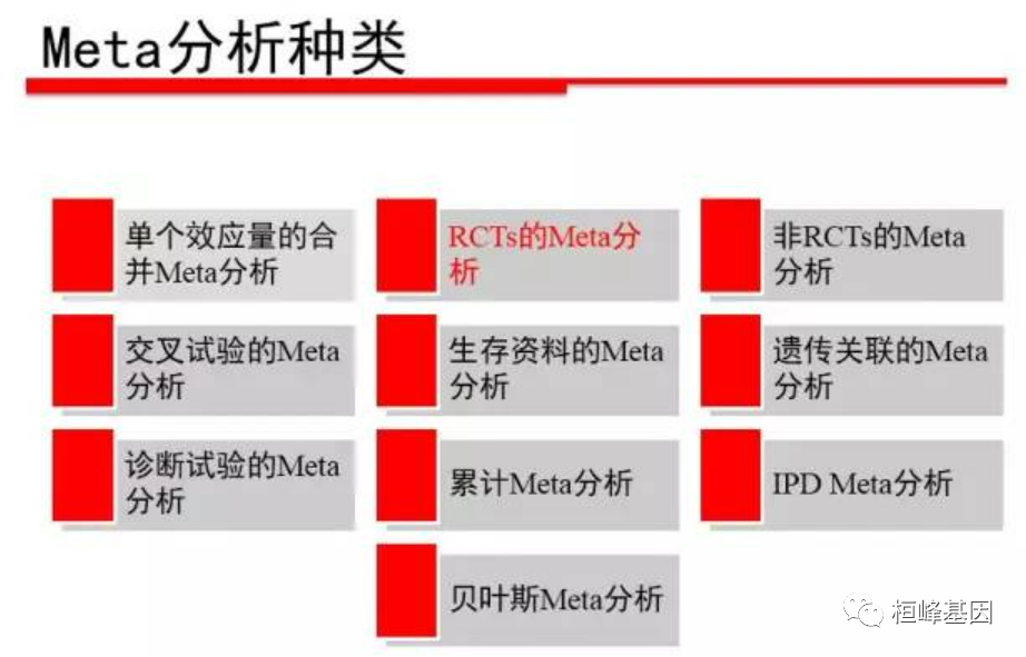
In 1976, Glass named this concept meta analysis for the first time. It is defined as a method of collecting, merging and statistical analysis of different research results. This method has gradually developed into a new discipline - "evidence-based medicine", the main content and research means. The main purpose of Meta-analysis is to comprehensively reflect the previous research results more objectively. Researchers do not conduct the original research, but comprehensively analyze the results obtained from the research.
02 input data mode
 We use R package metafor, developed by Viechtbauer, which can not only complete the Meta-analysis of binary classification and continuity variables, but also carry out regression analysis. This software package is the only package that can carry out the fitting operation of mixed effect model, including:
-
Single variable
-
Multi classification variable
-
Continuity variable
It can also detect the model coefficients and obtain the confidence interval, and accurately test the parameters, such as permutation test.
Package installation, as follows:
install.packages("metafor")
library("metafor")
The software package data were obtained from 13 studies that examined BCG's anti tuberculosis effects. The purpose of meta analysis was to examine the overall effectiveness of BCG in preventing TB and to examine possible mitigation agents. This data set has been used in some publications to illustrate the meta-analysis method, as follows:
data("dat.bcg")
print(dat.bcg, row.names = FALSE)
trial               author year tpos  tneg cpos  cneg ablat      alloc
     1              Aronson 1948    4   119   11   128    44     random
     2     Ferguson & Simes 1949    6   300   29   274    55     random
     3      Rosenthal et al 1960    3   228   11   209    42     random
     4    Hart & Sutherland 1977   62 13536  248 12619    52     random
     5 Frimodt-Moller et al 1973   33  5036   47  5761    13  alternate
     6      Stein & Aronson 1953  180  1361  372  1079    44  alternate
     7     Vandiviere et al 1973    8  2537   10   619    19     random
     8           TPT Madras 1980  505 87886  499 87892    13     random
     9     Coetzee & Berjak 1968   29  7470   45  7232    27     random
    10      Rosenthal et al 1961   17  1699   65  1600    42 systematic
    11       Comstock et al 1974  186 50448  141 27197    18 systematic
    12   Comstock & Webster 1969    5  2493    3  2338    33 systematic
    13       Comstock et al 1976   27 16886   29 17825    33 systematic

#######Data description
?dat.bcg
  Format
The data frame contains the following columns:

trial  numeric  trial number
author  character  author(s)
year  numeric  publication year
tpos  numeric  number of TB positive cases in the treated (vaccinated) group
tneg  numeric  number of TB negative cases in the treated (vaccinated) group
cpos  numeric  number of TB positive cases in the control (non-vaccinated) group
cneg  numeric  number of TB negative cases in the control (non-vaccinated) group
ablat  numeric  absolute latitude of the study location (in degrees)
alloc  character  method of treatment allocation (random, alternate, or systematic assignment)
The 13 studies provide data details in the following tables:
| TB positive | TB negative | |
| vaccinated group | tpos | tneg |
| control group | cpos | cneg |
03 example analysis
Calculate the log relative risk and the corresponding sampling variance as follows:
dat <- escalc(measure = "RR", ai = tpos, bi = tneg, ci = cpos,
              di = cneg, data = dat.bcg, append = TRUE)
print(dat[,-c(4:7)], row.names = FALSE
trial               author year ablat      alloc      yi     vi
     1              Aronson 1948    44     random -0.8893 0.3256
     2     Ferguson & Simes 1949    55     random -1.5854 0.1946
     3      Rosenthal et al 1960    42     random -1.3481 0.4154
     4    Hart & Sutherland 1977    52     random -1.4416 0.0200
     5 Frimodt-Moller et al 1973    13  alternate -0.2175 0.0512
     6      Stein & Aronson 1953    44  alternate -0.7861 0.0069
     7     Vandiviere et al 1973    19     random -1.6209 0.2230
     8           TPT Madras 1980    13     random  0.0120 0.0040
     9     Coetzee & Berjak 1968    27     random -0.4694 0.0564
    10      Rosenthal et al 1961    42 systematic -1.3713 0.0730
    11       Comstock et al 1974    18 systematic -0.3394 0.0124
    12   Comstock & Webster 1969    33 systematic  0.4459 0.5325
    13       Comstock et al 1976    33 systematic -0.0173 0.0714
The demo formula interface is as follows:
k <- length(dat.bcg$trial)
dat.fm <- data.frame(study = factor(rep(1:k, each = 4)))
dat.fm$grp <- factor(rep(c("T", "T", "C", "C"), k), levels = c("T", "C"))
dat.fm$out <- factor(rep(c("+", "-", "+", "-"), k), levels = c("+", "-"))
dat.fm$freq <- with(dat.bcg, c(rbind(tpos, tneg, cpos, cneg)))
dat.fm
   study grp out  freq
1      1   T   +     4
2      1   T   -   119
3      1   C   +    11
4      1   C   -   128
5      2   T   +     6
6      2   T   -   300
7      2   C   +    29
8      2   C   -   274
9      3   T   +     3
10     3   T   -   228
11     3   C   +    11
12     3   C   -   209
13     4   T   +    62
14     4   T   - 13536
15     4   C   +   248
16     4   C   - 12619
17     5   T   +    33
18     5   T   -  5036
19     5   C   +    47
20     5   C   -  5761
21     6   T   +   180
22     6   T   -  1361
23     6   C   +   372
24     6   C   -  1079
25     7   T   +     8
26     7   T   -  2537
27     7   C   +    10
28     7   C   -   619
29     8   T   +   505
30     8   T   - 87886
31     8   C   +   499
32     8   C   - 87892
33     9   T   +    29
34     9   T   -  7470
35     9   C   +    45
36     9   C   -  7232
37    10   T   +    17
38    10   T   -  1699
39    10   C   +    65
40    10   C   -  1600
41    11   T   +   186
42    11   T   - 50448
43    11   C   +   141
44    11   C   - 27197
45    12   T   +     5
46    12   T   -  2493
47    12   C   +     3
48    12   C   -  2338
49    13   T   +    27
50    13   T   - 16886
51    13   C   +    29
52    13   C   - 17825
- The random effect model is as follows:
#The default model is REML model random effect model using restricted maximum likelihood estimator
res <- rma(yi, vi, data = dat)
res
Random-Effects Model (k = 13; tau^2 estimator: REML)

tau^2 (estimated amount of total heterogeneity): 0.3132 (SE = 0.1664)
tau (square root of estimated tau^2 value):      0.5597
I^2 (total heterogeneity / total variability):   92.22%
H^2 (total variability / sampling variability):  12.86

Test for Heterogeneity:
Q(df = 12) = 152.2330, p-val < .0001

Model Results:

estimate      se     zval    pval    ci.lb    ci.ub
 -0.7145  0.1798  -3.9744  <.0001  -1.0669  -0.3622  ***

---
Signif. codes:  0 '***' 0.001 '**' 0.01 '*' 0.05 '.' 0.1 ' ' 1

res <- rma(ai = tpos, bi = tneg, ci = cpos,
           di = cneg, data = dat, measure = "RR")
res
Random-Effects Model (k = 13; tau^2 estimator: REML)

tau^2 (estimated amount of total heterogeneity): 0.3132 (SE = 0.1664)
tau (square root of estimated tau^2 value):      0.5597
I^2 (total heterogeneity / total variability):   92.22%
H^2 (total variability / sampling variability):  12.86

Test for Heterogeneity:
Q(df = 12) = 152.2330, p-val < .0001

Model Results:

estimate      se     zval    pval    ci.lb    ci.ub
 -0.7145  0.1798  -3.9744  <.0001  -1.0669  -0.3622  ***

---
Signif. codes:  0 '***' 0.001 '**' 0.01 '*' 0.05 '.' 0.1 ' ' 1
For the confidence interval of heterogeneity, the confidence interval of heterogeneity coefficient (tau2,tau,I2(%),H^2) can be calculated by confint () in metafor, as follows:
### confidence intervals for tau^2, I^2, and H^2

confint(res)
     estimate   ci.lb   ci.ub
tau^2    0.3132  0.1197  1.1115
tau      0.5597  0.3460  1.0543
I^2(%)  92.2214 81.9177 97.6781
H^2     12.8558  5.5303 43.0680
# Prediction / confidence interval of estimated effect quantity
predict(res, digits = 3)
 pred    se  ci.lb  ci.ub  pi.lb pi.ub
 -0.715 0.180 -1.067 -0.362 -1.867 0.438
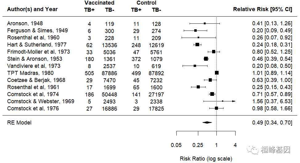
- forest map
Forest map is based on statistical indicators and statistical analysis methods and drawn with numerical calculation results. In the plane rectangular coordinate system, it takes a vertical invalid line (the abscissa scale is 1 or 0) as the center, uses multiple line segments parallel to the horizontal axis to describe the effect quantity and confidence interval of each research, and uses a prism (or other graphics) to describe the effect quantity and confidence interval of multiple research combinations. It is very simple and intuitive to describe the statistical results of Meta-analysis. It is the most commonly used result expression in Meta-analysis. As follows:
### forst plot
forest(res, slab = paste(dat$author, dat$year, sep = ", "),
       xlim = c(-16, 6), at = log(c(.05, .25, 1, 4)), atransf = exp,
       ilab = cbind(dat$tpos, dat$tneg, dat$cpos, dat$cneg),
       ilab.xpos = c(-9.5, -8, -6, -4.5), cex = .75)
op <- par(cex = .75, font = 2)
text(c(-9.5, -8, -6, -4.5), 15, c("TB+", "TB-", "TB+", "TB-"))
text(c(-8.75, -5.25),       16, c("Vaccinated", "Control"))
text(-16,                   15, "Author(s) and Year",     pos = 4)
text(6,                     15, "Relative Risk [95% CI]", pos = 2)
par(op)
The mixed effect model is as follows:
### mixed-effects model with absolute latitude and publication year as moderators
res <- rma(yi, vi, mods = cbind(ablat, year), data = dat)
res
Mixed-Effects Model (k = 13; tau^2 estimator: REML)
tau^2 (estimated amount of residual heterogeneity): 0.1108 (SE = 0.0845)
tau (square root of estimated tau^2 value): 0.3328
I^2 (residual heterogeneity / unaccounted variability): 71.98%
H^2 (unaccounted variability / sampling variability): 3.57
R^2 (amount of heterogeneity accounted for): 64.63%
Test for Residual Heterogeneity:
QE(df = 10) = 28.3251, p-val = 0.0016
Test of Moderators (coefficients 2:3):
QM(df = 2) = 12.2043, p-val = 0.0022
Model Results:
estimate se zval pval ci.lb ci.ub
intrcpt -3.5455 29.0959 -0.1219 0.9030 -60.5724 53.4814
ablat -0.0280 0.0102 -2.7371 0.0062 -0.0481 -0.0080 **
year 0.0019 0.0147 0.1299 0.8966 -0.0269 0.0307
---
Signif. codes: 0 '***' 0.001 '**' 0.01 '*' 0.05 '.' 0.1 ' ' 1
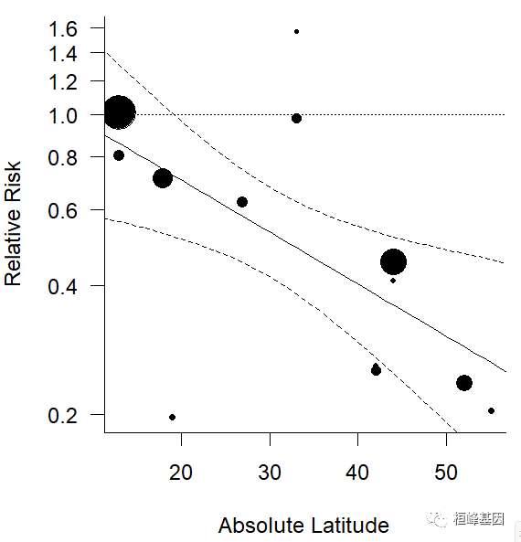
### predicted average relative risks for 10, 20, 30, 40, and 50 degrees
### absolute latitude holding publication year constant at 1970
predict(res, newmods = cbind(seq(from = 10, to = 60, by = 10), 1970),
transf = exp, addx = TRUE)
### plot of the predicted average relative risk as a function of absolute latitude
preds <- predict(res, newmods = cbind(0:60, 1970), transf = exp)
wi <- 1/sqrt(dat$vi)
size <- 0.5 + 3 * (wi - min(wi))/(max(wi) - min(wi))
plot(dat$ablat, exp(dat$yi), pch = 19, cex = size,
xlab = "Absolute Latitude", ylab = "Relative Risk",
las = 1, bty = "l", log = "y")
lines(0:60, preds$pred)
lines(0:60, preds$ci.lb, lty = "dashed")
lines(0:60, preds$ci.ub, lty = "dashed")
abline(h = 1, lty = "dotted")
- funnel diagram
Funnel chart is a scatter chart proposed by Light et al. In 1984, which generally takes the effect quantity of a single study as the abscissa and the sample content as the ordinate. The effect quantity can be RR, OR and death ratio OR its logarithm. Theoretically, the point estimation of each independent research effect included in Meta-analysis should be an inverted funnel shape in the plane coordinate system, so it is called funnel diagram.
-
The sample size is small and the research accuracy is low. It is distributed at the bottom of the funnel diagram and scattered around;
-
The sample size is large and the research accuracy is high. It is distributed at the top of the funnel diagram and concentrated in the middle.
In actual use, when the number of studies for Meta-analysis is small, it is not suitable to make a funnel chart. Generally, it is recommended that the funnel chart should be made only when the number of studies for Meta-analysis is 10 or more. Funnel chart is mainly used to observe whether there is bias in the results of a system evaluation or Meta-analysis, such as publication bias or other bias, as shown in the following figure:
### funnel plots
res <- rma(yi, vi, data = dat)
funnel(res, main = "Random-Effects Model")
res <- rma(yi, vi, mods = cbind(ablat), data = dat)
funnel(res, main = "Mixed-Effects Model")
#######Begger's test
ranktest(res)
Rank Correlation Test for Funnel Plot Asymmetry

Kendall's tau = 0.0256, p = 0.9524
##########Egger's test
regtest(res)
Regression Test for Funnel Plot Asymmetry

Model:     mixed-effects meta-regression model
Predictor: standard error

Test for Funnel Plot Asymmetry: z = -0.4623, p = 0.6439

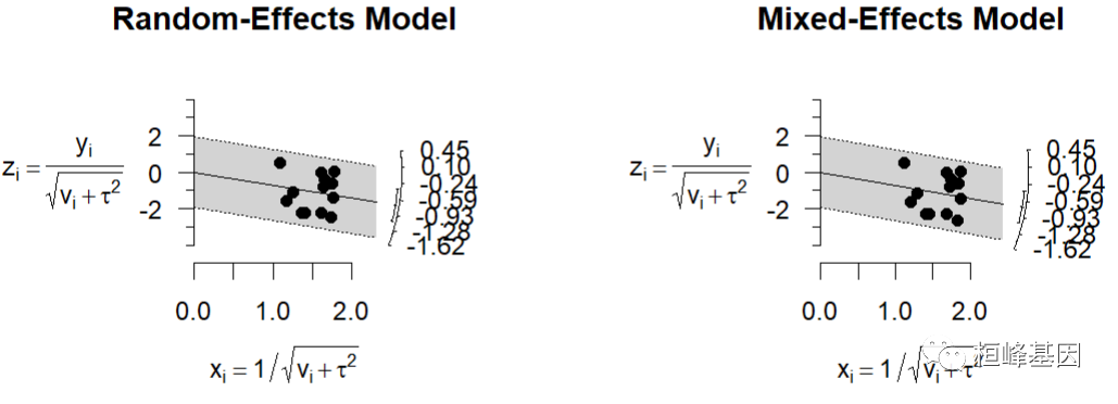
- radial star
It mainly reflects the heterogeneity of various studies, so as to find the points of heterogeneity. The effect corresponding to the arc is evaluated by size distribution. As follows:
### radial plots
res <- rma(yi, vi, data = dat, method = "REML")
radial(res, main = "Random-Effects Model")
res <- rma(yi, vi, data = dat, method = "ML")
radial(res, main = "Mixed-Effects Model")
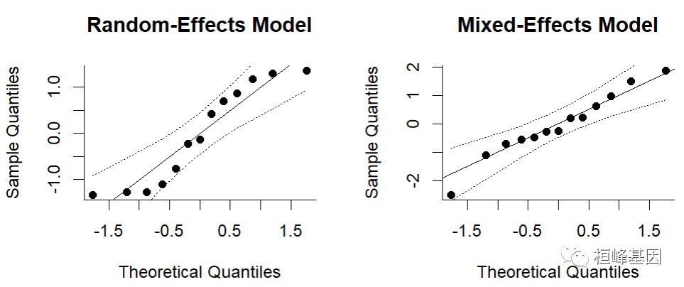
- Q-Q bitmap
Draw the prediction results and observe whether they are within the confidence interval, as follows:
### qq-normal plots
res <- rma(yi, vi, data = dat)
qqnorm(res, main = "Random-Effects Model")
res <- rma(yi, vi, mods = cbind(ablat), data = dat)
qqnorm(res, main = "Mixed-Effects Model")
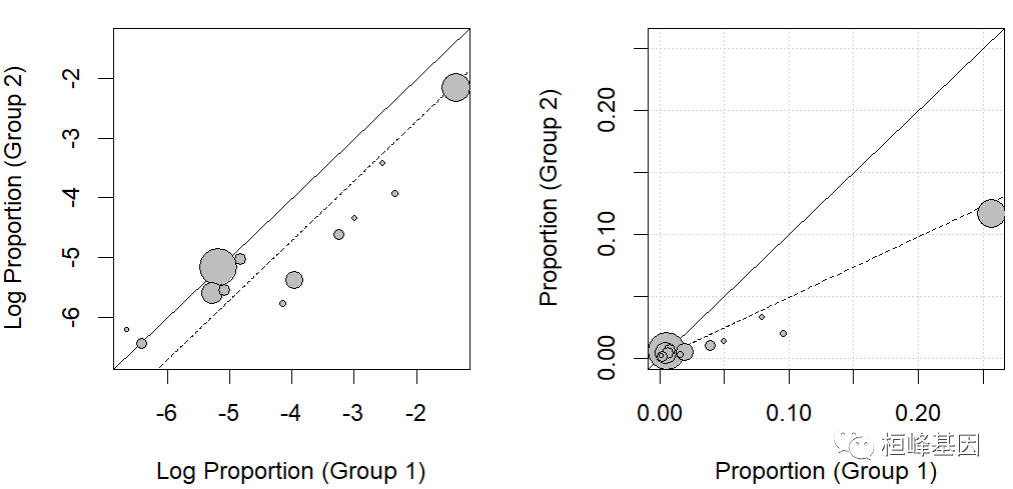
- labbe labetu
This function calculates the arm level results of the two groups (e.g., treatment and control) and compares them with each other. Incidence rate of incidence rate is incidence of the two groups of functional blocks, especially in the analysis of risk differences. The log odds ratio is analyzed in the log log log ratio. The log odds ratio is analyzed in the analysis of the odds ratio (log), the square root inverse sine transformation ratio is used to analyze the risk difference of the square root sine transform, and the incidence rate is analyzed with the original incidence rate, and the incidence ratio is analyzed by the logarithm of incidence (log). The square root conversion of incidence rate is analyzed as follows: incidence rate difference.
res <- rma(measure="RR", ai=tpos, bi=tneg, ci=cpos, di=cneg, data=dat.bcg)

### default plot
labbe(res)

### funnel plot with risk values on the x- and y-axis and add grid
labbe(res, transf=exp, grid=TRUE)
# }
04 interpretation of analysis results
It can be seen that I^2 is 71.98%, which belongs to high heterogeneity, and the random effect model can be used. When heterogeneity is low, fixed effect model and random effect model can be used, and the results are not different, but high heterogeneity can only choose random effect model, otherwise the extrapolation of results will be constrained. The random effect model is selected here for conservative consideration.
The random effect model is based on the assumption that there is heterogeneity across studies. The merger model recognizes the existence of heterogeneity among studies, but does not deal with heterogeneity; If there is heterogeneity among the studies included in the merger, although it does not reach the I ^ 2 > 50% we normally set, when merging with fixed effect model, the default operation directly ignores the existence of this part of heterogeneity, so the merger result will cause false positive error. When merging with random effect model, although the heterogeneity is not handled, However, its default operation recognizes the existence of heterogeneity, and the merging result is more reliable!
From the funnel chart and the results of Begg's test and Egger's test, we can see that the P value is greater than 0.05, which means there is no publication bias.
Meta analysis is also an option for publishing articles. To find out these diagrams and internal methods, as for the score of SCI, we still need to see the novelty of the subject we study, and the methods are basically these. As long as you have good data, it's just around the corner to publish a high score of SCI. In the next issue, we'll talk about other software!
Pay attention to the official account, scan the code into groups, free answers, and later there will be free live tutorials. Please look forward to it!
Reference:
-
Viechtbauer, W. (2010). Conducting Meta-Analyses in R with the metafor Package. Journal of Statistical Software, 36(3), 1–48.
-
Colditz, G. A., Brewer, T. F., Berkey, C. S., Wilson, M. E., Burdick, E., Fineberg, H. V., & Mosteller, F. (1994). Efficacy of BCG vaccine in the prevention of tuberculosis: Meta-analysis of the published literature. Journal of the American Medical Association, 271(9), 698–702.
-
Berkey, C. S., Hoaglin, D. C., Mosteller, F., & Colditz, G. A. (1995). A random-effects regression model for meta-analysis. Statistics in Medicine, 14(4), 395–411.
-
van Houwelingen, H. C., Arends, L. R., & Stijnen, T. (2002). Advanced methods in meta-analysis: Multivariate approach and meta-regression. Statistics in Medicine, 21(4), 589–624.
-
Viechtbauer, W. (2010). Conducting meta-analyses in R with the metafor package. Journal of Statistical Software, 36(3), 1–48.

Huanfeng gene
Bioinformatics analysis, SCI article writing and bioinformatics basic knowledge learning: R language learning, perl basic programming, linux system commands, Python meet you better
34 original content
official account
