The data used in this example is three categories of English data. torchtext is used to process the data, build an iterator and build textcnn. The data is trained with textcnn to get the training results. In this example, the validation set is not used to evaluate the model.
1, Development environment and data set
1. Development environment
Ubuntu 16.04.6
python: 3.7
pytorch: 1.8.1
torchtext: 0.9.1
2. Data set
Dataset: train_data_sentiment
Extraction code: gw77
2, Working with datasets using torchtext
1. Import necessary Libraries
#Import common library
import torch
import pandas as pd
import matplotlib.pyplot as plt
from gensim.models import KeyedVectors
import torch.nn as nn
import torch.optim as optim
import torch.utils.data as Data
import torch.nn.functional as F
import torchtext
#Torchtext. Is required to compare the latest version legacy. Data, the old version of torchtext uses torchtex data
from torchtext.legacy.data import TabularDataset
import warnings
warnings.filterwarnings("ignore")
device = torch.device("cuda:1" if torch.cuda.is_available() else "cpu") #When I was writing my blog, our lab server 3 card was not used, so I used 3 card
2. Import and view datasets
#When you build a Dataset, you can also directly import the Dataset later
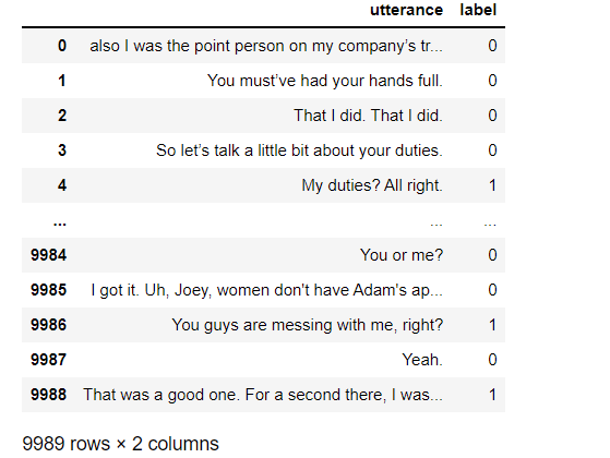
train_data = pd.read_csv('train_data_sentiment.csv')
train_data
3. Working with datasets using torchtext
Torchtext's data processing mainly includes three parts: defining Field, Dataset and iterator. It can easily process text data, such as word segmentation, truncation and length supplement, construction of thesaurus, etc. If you are not familiar with torchtext, you can learn the official documents or explain the blog.
3.1. Define Field
TEXT = torchtext.legacy.data.Field(sequential=True,lower=True,fix_length=30)#The default word breaker is split(), space division
LABEL = torchtext.legacy.data.Field(sequential=False,use_vocab=False)
- sequential: whether to represent the data as a sequence. If False, word segmentation cannot be used. Default: True.
- lower: whether to convert data to lowercase. Default: False.
- fix_length: when building the iterator, modify the length of each text data to this value, truncate and supplement the length, and use pad_ Complete the token. Default: None.
- use_vocab: whether to use dictionary objects If False, the data type must already be numeric. Default: True.
3.2. Define Dataset
TabularDataset can easily read data files in CSV, JSON or TSV format.
train_x = TabularDataset(path = 'train_data_sentiment.csv',
                        format = 'csv',skip_header=True,
                        fields = [('utterance',TEXT),('label',LABEL)])
- skip_header = True, column names are not treated as data.
- The order of fields should be the same as that of the original data columns.
You can see that the text data has been segmented

3.3. Build thesaurus and load pre training word vector
Because the computer doesn't know the text, we need to convert the text data into values or vectors, so that we can input it into textcnn or deep neural network for training. Firstly, the text data is constructed into the form of word index. Then, after loading the pre trained word vector, each word will correspond to a word vector, that is, the form of word vector. Finally, in the later model training, we can use the word Embedding matrix, that is, the Embedding layer. In this way, we can convert each word into a vector, which can be input into the model for training.
Here I will explain the word embedding matrix, because it takes me a long time to understand the word embedding matrix when I study. After we build the thesaurus, we can use the index to represent a sentence. According to the thesaurus built below, for example, it is you, this sentence can be represented by 109 3. Of course, we can directly use the index to input into the network for training, but the index represents too few features, In order to get better features to train the network, we usually use word2vec vector or glove vector. In this paper, glove vector is used, so that the features of each word can be better represented, which is more conducive to our training network. Each word in it is you will be represented by a 300 dimensional vector, which will input more features into the network, and our network model will be trained better. Summarize the word embedding matrix, that is: ① build a word list, that is, word index; ② Load the pre training word vector, i.e. word vector; ③ The word embedding matrix, i.e. index vector, is obtained.
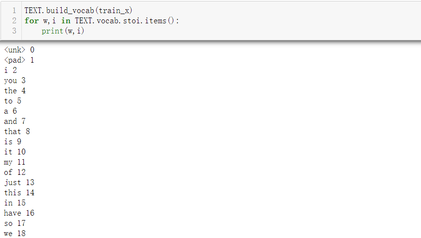
#Build Thesaurus
TEXT.build_vocab(train_x) #10440 words were constructed from 0-10439
for w,i in TEXT.vocab.stoi.items():
    print(w,i)
#Load the glove word vector, and it will be downloaded automatically for the first time. You can also download the word vector yourself. I use 400000 words here, and each word is represented by a 300 dimensional vector
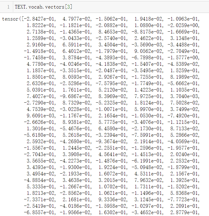
TEXT.vocab.load_vectors('glove.6B.300d',unk_init=torch.Tensor.normal_) #Randomly initialize the words that exist in the data but do not exist in the glove word vector and allocate a 300 dimensional vector
We can check the vectors in the built word embedding matrix. Here is the word vector with index 3 in the vocabulary we built, that is, the word you. Of course, this word is represented by a 300 dimensional vector. Here is only a screenshot.
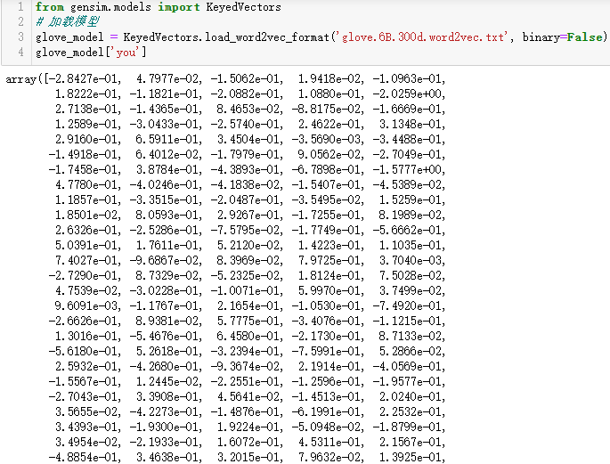
Let's take another look at the vector corresponding to the word you in the glove vector. Here is only part of the screenshot, which shows that we can obtain the vector of the corresponding word through the index, that is, the meaning of the word embedding matrix.
#View word vector dimension
print(TEXT.vocab.vectors.shape) #torch.Size([10440, 300])
It can be seen that our data is divided into 10440 words, each word is represented by a 300 dimensional vector, and then we can build an iterator.
3.4. Building iterators
Iterators include Iterator and bucket Iterator
- Iterator: build batch data in the same order as the original data.
- Bucket iterator: build data with similar length into a batch of data, which will reduce the filling during truncation and lengthening.
Generally, when training the network, we will input a batch data every time. I set batch_size=64, then there are 9989 / / 64 + 1 = 157 batches, because we have a total of 9989 data, each batch has 64 data, and 9989 / 64 = 156, then the remaining 5 data will form a batch.
batch_size = 64
train_iter = torchtext.legacy.data.Iterator(dataset = train_x,batch_size=64,shuffle=True,sort_within_batch=False,repeat=False,device=device)
len(train_iter) #157
- shuffle: whether to disturb the data
- sort_within_batch: whether to sort the data in each batch
- Repeat: whether to repeat the iterative batch data in different epoch s
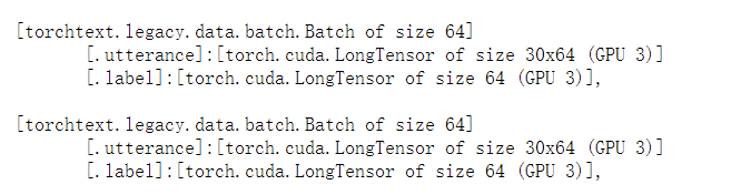
View the built iterator and the internal data representation:
#View built iterators
list(train_iter)
#View the size of batch data
for batch in train_iter:
    print(batch.utterance.shape)
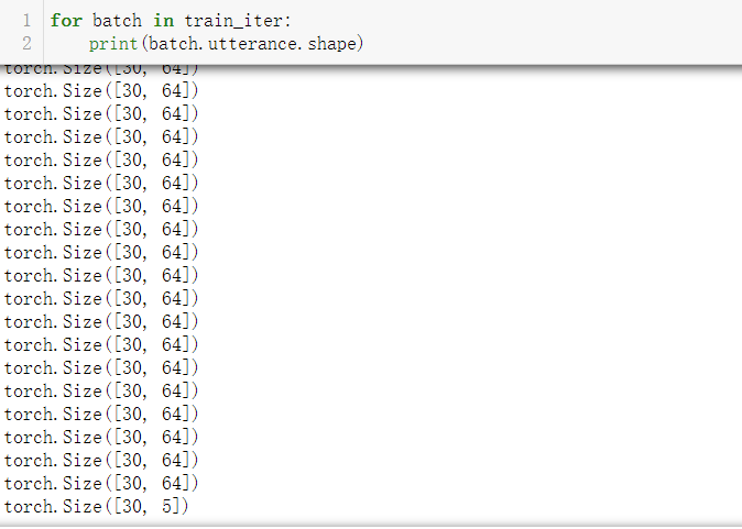
You can see that there are 64 pieces of data in each batch (except the last batch of data), that is, batch_size=64, each data consists of 30 words. We can also see that the last 5 data constitute a batch.
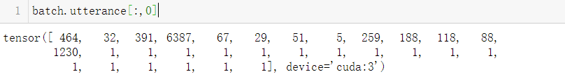
#View the first data
batch.utterance[:,0]#We take column 1, because column 1 represents the first data, that is, column 64 represents the 64th data. Each data consists of 30 words. The following non-1 part represents the index of the words in the first data in the thesaurus, and the remaining 1 represents the supplemented part.
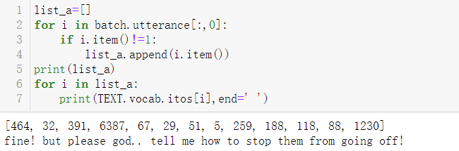
#View the index value corresponding to the word in the first data
list_a=[]
for i in batch.utterance[:,0]:
    if i.item()!=1:
        list_a.append(i.item())
print(list_a)
for i in list_a:
    print(TEXT.vocab.itos[i],end=' ')
#View the data in the iterator and its corresponding text
l =[]
for batch in list(train_iter)[:1]:
    for i in batch.utterance:
        l.append(i[0].item())
    print(l)
    print(' '.join([TEXT.vocab.itos[i] for  i in l]))

So far, the data has been processed. Next, let's learn about textcnn.
3, textcnn knowledge and pytorch framework construction
1. textcnn knowledge
textcnn is similar to cnn which is familiar with image processing, but the size of convolution kernel in cnn is generally k * k, while the size of convolution kernel in NLP is generally k * embedding_size, where embedding_size use embding for each word_ Word vector representation of size dimension. For example, a sentence in the figure below is composed of three words, and each word is represented by a three-dimensional word vector. We select two convolution kernels with the size of 2 * 3 to obtain the following results. The pooled results will actually be spliced. There is no splicing here for demonstration.
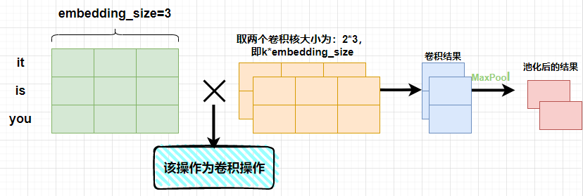
As can be seen from the above figure, the result obtained after convolution of a convolution kernel is [len (sense) - K + 1,1], where len (sense) represents the number of words in a sentence. After pooling, the result of [2,1] will be obtained. This result is spliced.
After understanding the basic theoretical knowledge, we can build the network framework of textcnn. If you want to know more about textcnn, you can find materials to continue learning.
2. Using pytorch to build textcnn
I built a two-tier textcnn network. The framework of textcnn is mainly: convolution, activation and pooling.
Parameter description in network framework:
- vocab_size: number of words in the constructed Thesaurus
- embedding_size: word vector dimension of each word
- num_channels: the number of output channels, that is, the number of convolution kernels
- kernel_sizes: convolution kernel size
kernel_sizes, nums_channels =  [3, 4], [150, 150]
embedding_size = 300
num_class = 3
vocab_size = 10440
Here I build a two-layer textcnn network. The size of the convolution core of the first layer is 3 * 300, and there are 150 convolution cores with the same shape. The size of the convolution core of the second layer is 4 * 300. Similarly, there are 150 such convolution cores. The textcnn framework code is as follows:
class TextCNN(nn.Module):
    def __init__(self,kernel_sizes,num_channels):
        super(TextCNN,self).__init__()
        self.embedding = nn.Embedding(vocab_size,embedding_size) #embedding layer
        self.dropout = nn.Dropout(0.5)
        self.convs = nn.ModuleList()
        for c,k in zip(num_channels,kernel_sizes):
            self.convs.append(nn.Sequential(nn.Conv1d(in_channels=embedding_size,
                                       out_channels = c,            #Here, the number of output channels is [150150], that is, there are 150 convolution kernels with a size of 3*embedding_size and 4 * embedding_ Convolution kernel of size
                                       kernel_size = k),            # The size of convolution kernel, here refers to 3 and 4
                             nn.ReLU(),                             #Activation function
                             nn.MaxPool1d(30-k+1)))                 #Pooling: select a maximum value from the 30-k+1 results after convolution. Each data represented by 30 is composed of 30 words,
        self.decoder = nn.Linear(sum(num_channels),3)               #In the full connection layer, the input is a 300 dimensional vector and the output is a 3-dimensional, that is, the number of classifications

    def forward(self,inputs):
        embed = self.embedding(inputs)   #[30,64,300]
        embed = embed.permute(1,2,0)     #[64300,30], this step is to exchange dimensions in order to comply with the input of the subsequent convolution operation
        #In the next encoding step, after two layers of textcnn, each layer will get a result of [64150,1], followed by [64150] after squeeze, and then splice the two results to get [64300]
        encoding = torch.cat([conv(embed).squeeze(-1) for conv in self.convs],dim=1) #[64,300]
        outputs =self.decoder(self.dropout(encoding))   #Input [64300] to the full connection layer, and finally get the result of [64,3]
        return outputs
Let's take a look at the built network framework
net = TextCNN(kernel_sizes, nums_channels).to(device)
net
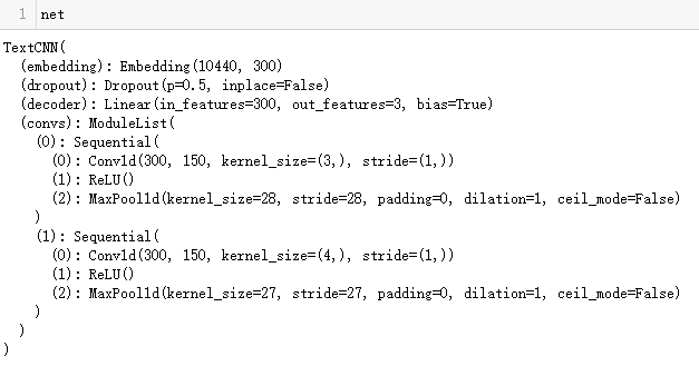
As can be seen from the figure, the network has two layers. The difference between these two layers is that the size of convolution kernel and pooling layer are different, and the others are the same.
- Enter the number of channels in_channels=300;
- Number of output channels out_channels=150;
- Convolution kernel size: the first layer is 3 * 300, and the second layer is 4 * 300
- The step size of convolution is stripe = 1
- The step size of the pool layer is stripe = 30 kernel_ Size + 1, because each data set consists of 30 words, the purpose of pooling is to select the largest value from the results after convolution, which is the purpose of maximum pooling, and the result after convolution is [30 kernel_size + 1,1]. You can push this step yourself, which is very simple.
4, Model training and results
1. Define parameters such as training function, optimizer and loss function
Generally, I define the training function and call it for model training. You can operate it at will.
net.embedding.weight.data.copy_(TEXT.vocab.vectors)    #Pass in our word Embedding matrix to the Embedding layer of the model
optimizer = optim.Adam(net.parameters(),lr=1e-4)       #Define the optimizer. lr is the learning rate, which can be adjusted by yourself
criterion = nn.CrossEntropyLoss().to(device)           #Define loss function
train_x_len = len(train_x)                             #This step is the amount of data I obtained to calculate the following Acc, that is, 9989
#Define training function
def train(net,iterator,optimizer,criterion,train_x_len):
    epoch_loss = 0                           #Initialize loss value
    epoch_acc = 0                            #Initialize acc value
    for batch in iterator:
        optimizer.zero_grad()                #Gradient clearing
        preds = net(batch.utterance)         #Forward propagation to obtain the predicted value
        loss = criterion(preds,batch.label)  #Calculate loss
        epoch_loss +=loss.item()             #Accumulate loss as the numerator of the average loss below
        loss.backward()                      #Back propagation
        optimizer.step()                     #Update weight parameters in the network
        epoch_acc+=((preds.argmax(axis=1))==batch.label).sum().item()   #Accumulate acc as the molecule for averaging acc below
    return epoch_loss/(train_x_len),epoch_acc/train_x_len    #The values returned are loss and acc
2. Conduct training
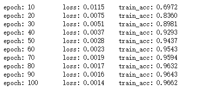
A total of 100 rounds of training were conducted, and printouts were conducted every 10 rounds.
n_epoch = 100
acc_plot=[]     #For drawing later
loss_plot=[]    #For drawing later
for epoch in range(n_epoch):
    train_loss,train_acc = train(net,train_iter,optimizer,criterion,train_x_len)
    acc_plot.append(train_acc)
    loss_plot.append(train_loss)
    if (epoch+1)%10==0:
        print('epoch: %d \t loss: %.4f \t train_acc: %.4f'%(epoch+1,train_loss,train_acc))
The results are as follows:
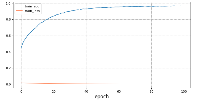
3. Visualization results
#Using the drawing function matplotlib
plt.figure(figsize =(10,5),dpi=80)
plt.plot(acc_plot,label='train_acc')
plt.plot(loss_plot,color='coral',label='train_loss')
plt.legend(loc = 0)
plt.grid(True,linestyle = '--',alpha=1)
plt.xlabel('epoch',fontsize = 15)
plt.show()
5, Summary
This paper mainly uses torchtext to process the training data set and construct it as an iterator for model input. It does not use the verification set to evaluate the model. You can try to separate the verification set from the training set to evaluate the model. The complete code is as follows:
#I have tested the code and there is no problem. I commented out some code for printout,
#Import common library
import torch
import pandas as pd
import matplotlib.pyplot as plt
from gensim.models import KeyedVectors
import torch.nn as nn
import torch.optim as optim
import torch.utils.data as Data
import torch.nn.functional as F
import torchtext
#Torchtext. Is required to compare the latest version legacy. Data, the old version of torchtext uses torchtex data
from torchtext.legacy.data import TabularDataset
import warnings
warnings.filterwarnings("ignore")
device = torch.device("cuda:1" if torch.cuda.is_available() else "cpu") #When I was writing my blog, our lab server 3 card was not used, so I used 3 card

train_data = pd.read_csv('train_data_sentiment.csv')
# train_data

#Processing data using torchtext
#Define filed
TEXT = torchtext.legacy.data.Field(sequential=True,lower=True,fix_length=30)
LABEL = torchtext.legacy.data.Field(sequential=False,use_vocab=False)

train_x = TabularDataset(path = 'train_data_sentiment.csv',
                        format = 'csv',skip_header=True,
                        fields = [('utterance',TEXT),('label',LABEL)])

# print(train_x[0].utterance)
# print(train_x[0].label)

TEXT.build_vocab(train_x)
# for w,i in TEXT.vocab.stoi.items():
#     print(w,i)

TEXT.vocab.load_vectors('glove.6B.300d',unk_init=torch.Tensor.normal_)

glove_model = KeyedVectors.load_word2vec_format('glove.6B.300d.word2vec.txt', binary=False)
# glove_model['you']

# print(TEXT.vocab.vectors.shape) #torch.Size([10440, 300])

batch_size = 64
train_iter = torchtext.legacy.data.Iterator(dataset = train_x,batch_size=64,shuffle=True,sort_within_batch=False,repeat=False,device=device)

# len(train_iter)
# list(train_iter)

# for batch in train_iter:
#     print(batch.utterance.shape)

# batch.utterance[:,0]

# list_a=[]
# for i in batch.utterance[:,0]:
#     if i.item()!=1:
#         list_a.append(i.item())
# print(list_a)
# for i in list_a:
#     print(TEXT.vocab.itos[i],end=' ')

# l =[]
# for batch in list(train_iter)[:1]:
#     for i in batch.utterance:
#         l.append(i[0].item())
#     print(l)
#     print(' '.join([TEXT.vocab.itos[i] for  i in l]))

kernel_sizes, nums_channels =  [3, 4], [150, 150]
embedding_size = 300
num_class = 3
vocab_size = 10440

#Build textcnn
class TextCNN(nn.Module):
    def __init__(self,kernel_sizes,num_channels):
        super(TextCNN,self).__init__()
        self.embedding = nn.Embedding(vocab_size,embedding_size)
        self.dropout = nn.Dropout(0.5)
        self.convs = nn.ModuleList()
        for c,k in zip(num_channels,kernel_sizes):
            self.convs.append(nn.Sequential(nn.Conv1d(in_channels=embedding_size,
                                       out_channels = c,
                                       kernel_size = k),
                             nn.ReLU(),
                             nn.MaxPool1d(30-k+1)))
        self.decoder = nn.Linear(sum(num_channels),3)
    def forward(self,inputs):
        embed = self.embedding(inputs)
        embed = embed.permute(1,2,0)
        encoding = torch.cat([conv(embed).squeeze(-1) for conv in self.convs],dim=1)
        outputs =self.decoder(self.dropout(encoding))
        return outputs

net = TextCNN(kernel_sizes, nums_channels).to(device)
# net

net.embedding.weight.data.copy_(TEXT.vocab.vectors)
optimizer = optim.Adam(net.parameters(),lr=1e-4)
criterion = nn.CrossEntropyLoss().to(device)
train_x_len = len(train_x)

#Define training function
def train(net,iterator,optimizer,criterion,train_x_len):
    epoch_loss = 0
    epoch_acc = 0
    for batch in iterator:
        optimizer.zero_grad()
        preds = net(batch.utterance)
        loss = criterion(preds,batch.label)
        epoch_loss +=loss.item()
        loss.backward()
        optimizer.step()
        epoch_acc+=((preds.argmax(axis=1))==batch.label).sum().item()
    return epoch_loss/(train_x_len),epoch_acc/train_x_len

n_epoch = 100
acc_plot=[]
loss_plot=[]
for epoch in range(n_epoch):
    train_loss,train_acc = train(net,train_iter,optimizer,criterion,train_x_len)
    acc_plot.append(train_acc)
    loss_plot.append(train_loss)
    if (epoch+1)%10==0:
        print('epoch: %d \t loss: %.4f \t train_acc: %.4f'%(epoch+1,train_loss,train_acc))

plt.figure(figsize =(10,5),dpi=80)
plt.plot(acc_plot,label='train_acc')
plt.plot(loss_plot,color='coral',label='train_loss')
plt.legend(loc = 0)
plt.grid(True,linestyle = '--',alpha=1)
plt.xlabel('epoch',fontsize = 15)
plt.show()