Description of several problems in generating countermeasure networks

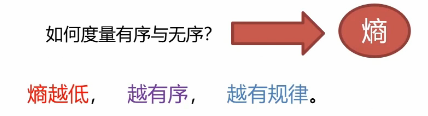
What is information entropy?

We use entropy to measure whether the data is ordered or disordered

Calculating information entropy

Information entropy is a measure of system chaos:

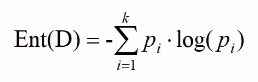
Where Pi represents the probability of an event, the minimum information entropy is 0, which indicates complete determination, the maximum is log (probability is 1), and it indicates that all situations may occur (completely disordered)

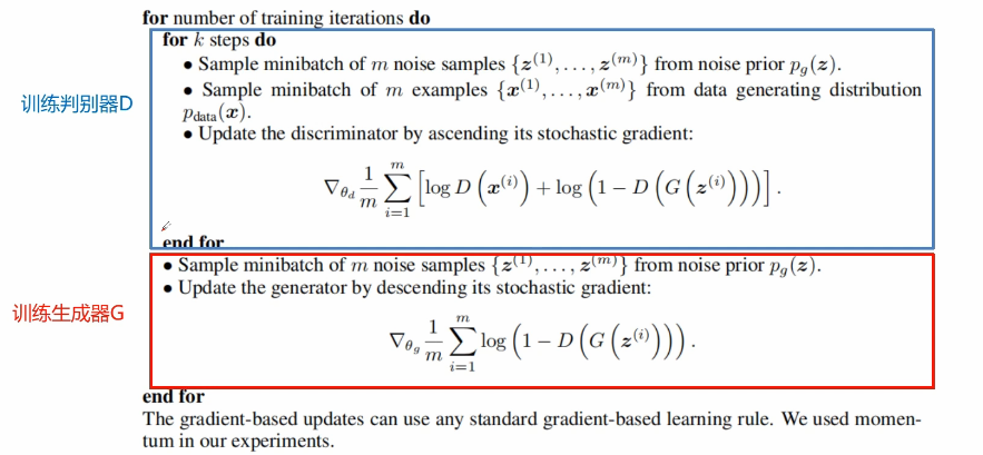
Countermeasure network loss function

The formula of the best discriminator is as follows

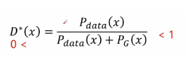
JS divergence can be obtained by bringing D * (x) into the cross entropy loss function (see the first blog on GAN for the specific derivation process):

Least Squares GAN(LSGAN)

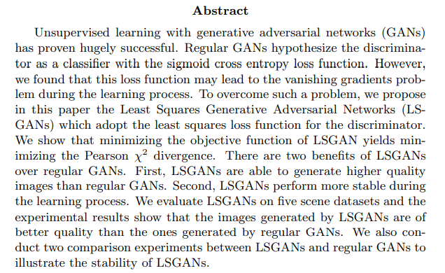
Through the original paper abstract, we can extract the following key information:
Previous studies have proved that GAN network is very good. For ordinary GAN network, the discriminator uses a Sigmoid activation function as a classifier to carry out the relationship of cross entropy loss function. In order to overcome this problem, we use the minimum mean square error loss function to replace the cross entropy loss function.
To sum up: the task of LSGAN is to replace Sigmoid activation function with linear activation function (regression task instead of classification task)

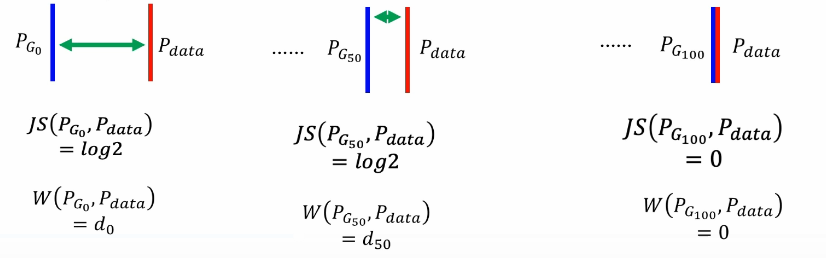
JS divergence problem -- immeasurable

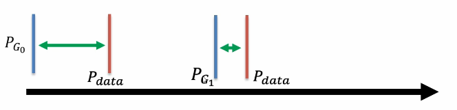
JS divergence is used to measure the distance between generated data and real data. However, no matter what the two distances are, JS divergence is always Log2 as long as they do not overlap. JS divergence is 0 only when the two data coincide. Obviously, when the two distributions do not overlap, the accuracy rate of secondary classification has always been 100%. There is no way to distinguish a good degree, so it has no practical significance.

Wasserstein GAN(WGAN)

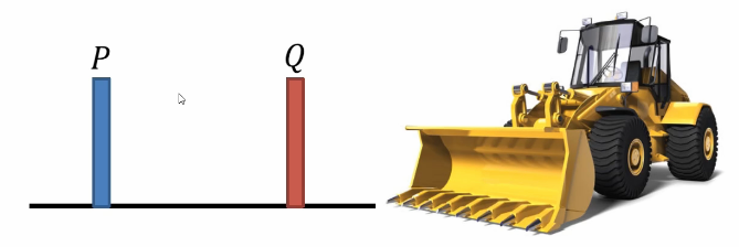
Earth Mover "s Distance:
Suppose distribution p is a piece of soil and another distribution q is the target. The bulldozing distance is the average distance to push a piece of soil p to Q.

WGAN bulldozing distance

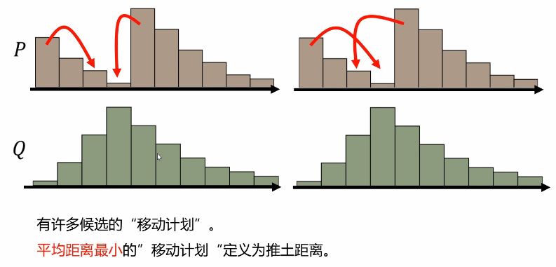
Find the best shoveling strategy

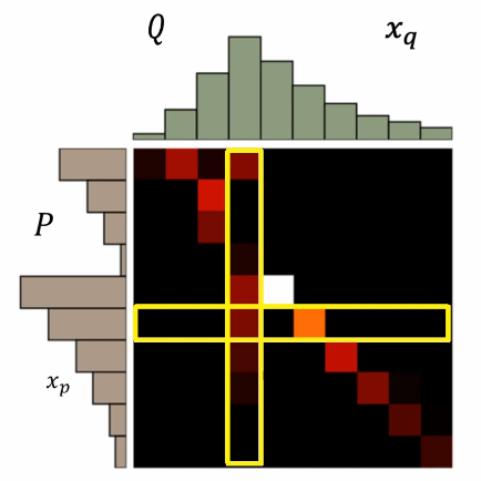
A "move plan" is a matrix in which each element is the amount moved from one location to another

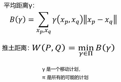
Bulldozing distance: list all Π， Choose the smallest γ As an optimal strategy

Smoothing measure

For JS divergence to describe the distance between data distributions, here we use bulldozer distance to measure the following better and smoother measurement effect

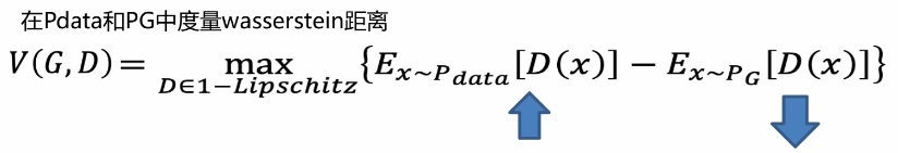
WGAN loss function

In WGAN, the discriminator does not need to be marked as 0 and 1. It only needs to output positive numbers for real data and negative numbers for forged data. And the discriminator d must smooth the constraint. If there is no constraint, the training of discriminator D will not converge. So how do you implement this constraint?

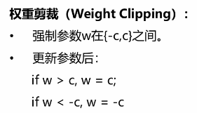
Weight clipping

Conditions for smooth constraint implementation:

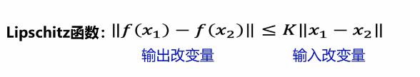
For the problem raised in the previous section, in fact, the gradient should not be too limited, and a scheme such as weight clipping is adopted.

Improved GAN(WGAN—GP)

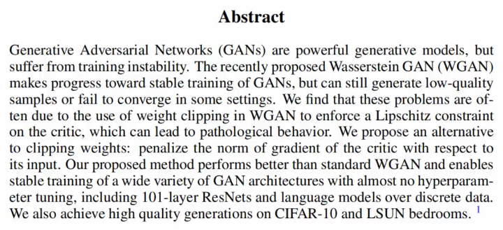
The following key information can be obtained from reading the abstract of the original WGAN-GP paper:
WGAN further improves the stability of training, but it will still produce some low-quality data or convergence errors in some settings. The author of this article found that the frequent use of weight clipping may lead to some wrong problems. Therefore, the author proposed the penalty gradient standard deviation method to replace weight clipping to achieve a better effect.

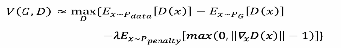
WGAN-GP loss function

In short, this constraint is added to the total loss function. Such a penalty term is called gradient penalty, as follows:

WGAN - GP constraint penalty

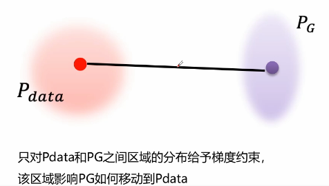
For the connection between the two distributions of real data and generated data, the average value can be taken as the constrained data. Only by giving gradient constraints to the distribution of the region between real data and generated data, can the region affect how Pg affects Pdata. The process of moving step by step, constantly taking the average value and constantly moving, then the data in this section is called penalty data. The maximum gradient in this region is equal to 1. Relevant experiments show that this method converges faster and better,

WGAN algorithm steps

EBGAN

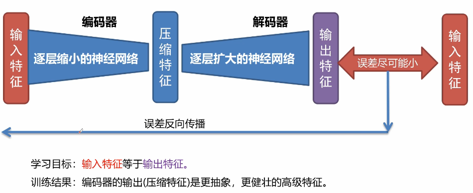
Introduction to automatic encoder

The automatic encoder can be understood as such a symmetrical structure

EBGAN network structure

The better an image can be reconstructed, the higher its quality. In EBGAN, automatic encoder is the most discriminator D. The network structure of the generator remains unchanged. For the discriminator, the input is a real image. After training by the automatic encoder, the quality of the image can be determined by constructing the loss. The advantage is that the pre training is only carried out through the real image without the generator. Unlike the traditional GAN training, there is no need for the interaction between the generator and the discriminator to distinguish a binary classification problem. For EBGAN, the real data has been compressed and reconstructed, and then the data of the generator is put into the discriminator to judge the effect of the generated data according to the loss.

Coding of main network modules

Initialization discriminator code

 def _init_discriminator(self, input, isTrain=True, reuse=False):
        """
        Initialization discriminator
        :param input:input data op
        :param isTrain: Training status
        :param reuse: Reusable variable
        :return: judge op
        """
        with tf.variable_scope('discriminator', reuse=reuse):
            # hidden layer 1 input =[none,64,64,3]
            conv1 = tf.layers.conv2d(input, 32, [3, 3], strides=(2, 2), padding='same')  # [none,32,32,32]
            bn1 = tf.layers.batch_normalization(conv1, training=isTrain)
            active1 = tf.nn.leaky_relu(bn1)  # [none,32,32,32]
            # hidden 2
            conv2 = tf.layers.conv2d(active1, 64, [3, 3], strides=(2, 2), padding='same')  # [none,16,16,64]
            bn2 = tf.layers.batch_normalization(conv2, training=isTrain)
            active2 = tf.nn.leaky_relu(bn2)  # [none,16,16,64]
            # hidden 3
            conv3 = tf.layers.conv2d(active2, 128, [3, 3], strides=(2, 2), padding="same")  # [none,8,8,128]
            bn3 = tf.layers.batch_normalization(conv3, training=isTrain)
            active3 = tf.nn.leaky_relu(bn3)  # [none,8,8,128]
            # hidden 4
            conv4 = tf.layers.conv2d(active3, 256, [3, 3], strides=(2, 2), padding="same")  # [none,4,4,256]
            bn4 = tf.layers.batch_normalization(conv4, training=isTrain)
            active4 = tf.nn.leaky_relu(bn4)  # [none,4,4,256]
            # out layer
            out_logis = tf.layers.conv2d(active4, 1, [4, 4], strides=(1, 1), padding='valid')  # [none,1,1,1]
        return out_logis
;

Initialize generator code

// An highlighted block
    def _init_generator(self, input, isTrain=True, reuse=False):
        """
        Initialize generator
        :param input:input op
        :param isTrain: Training status
        :param reuse: Reuse variables
        :return: Generate data op
        """
        with tf.variable_scope('generator', reuse=reuse):
            # input [none,1,noise_dim]
            conv1 = tf.layers.conv2d_transpose(input, 512, [4, 4], strides=(1, 1), padding="valid")  # [none,4,4,512]
            bn1 = tf.layers.batch_normalization(conv1, training=isTrain)
            active1 = tf.nn.leaky_relu(bn1)  # [none,4,4,512]
            # deconv layer 2
            conv2 = tf.layers.conv2d_transpose(active1, 256, [3, 3], strides=(2, 2), padding="same")  # [none,8,8,256]
            bn2 = tf.layers.batch_normalization(conv2, training=isTrain)
            active2 = tf.nn.leaky_relu(bn2)  # [none,8,8,256]
            # deconv layer 3
            conv3 = tf.layers.conv2d_transpose(active2, 128, [3, 3], strides=(2, 2), padding="same")  # [none,16,16,128]
            bn3 = tf.layers.batch_normalization(conv3, training=isTrain)
            active3 = tf.nn.leaky_relu(bn3)  # [none,16,16,128]
            # deconv layer 4
            conv4 = tf.layers.conv2d_transpose(active3, 64, [3, 3], strides=(2, 2), padding="same")  # [none,32,32,64]
            bn4 = tf.layers.batch_normalization(conv4, training=isTrain)
            active4 = tf.nn.leaky_relu(bn4)  # [none,32,32,64]
            # out layer
            conv5 = tf.layers.conv2d_transpose(active4, 3, [3, 3], strides=(2, 2), padding="same")  # [none,64,64,3]
            out = tf.nn.tanh(conv5)
        return out;

Key code of initialization training method

   def _init_train_methods(self):
        """
        Initialization training method: generator and discriminator loss, gradient descent method, initialization session. 
        :return: None
        """
        # Find the variables related to the generator and discriminator
        total_vars = tf.trainable_variables()
        d_vars = [var for var in total_vars if var.name.startswith("discriminator")]
        g_vars = [var for var in total_vars if var.name.startswith("generator")]
        if self.mode == "lsgan":
            self._init_lsgan_loss()
            self.D_trainer = tf.train.RMSPropOptimizer(learning_rate=1e-4).minimize(self.D_loss, var_list=d_vars)
            self.G_trainer = tf.train.RMSPropOptimizer(learning_rate=1e-4).minimize(self.G_loss, var_list=g_vars)
        elif self.mode == "wgan":
            self._init_wgan_loss()
            self.clip_d = [p.assign(tf.clip_by_value(p, -0.1, 0.1)) for p in d_vars]
            self.D_trainer = tf.train.RMSPropOptimizer(learning_rate=5e-5).minimize(self.D_loss, var_list=d_vars)
            self.G_trainer = tf.train.RMSPropOptimizer(learning_rate=5e-5).minimize(self.G_loss, var_list=g_vars)
        elif self.mode == "wgan-gp":
            self._init_wgan_gp_loss()
            self.D_trainer = tf.train.AdamOptimizer(
                learning_rate=1e-4, beta1=0., beta2=0.9).minimize(self.D_loss, var_list=d_vars)
            self.G_trainer = tf.train.AdamOptimizer(
                learning_rate=1e-4, beta1=0., beta2=0.9).minimize(self.G_loss, var_list=g_vars)
        # Initialize Session
        self.sess = tf.InteractiveSession()
        self.sess.run(tf.global_variables_initializer())
        self.saver = tf.train.Saver(max_to_keep=1);

DCGAN loss function initialization code

// An highlighted block
    def _init_dcgan_loss(self):
        # Initialize DCGAN loss function
        self.D_loss_real = tf.reduce_mean(
            tf.nn.sigmoid_cross_entropy_with_logits(logits=self.real_logis, labels=tf.ones_like(self.real_logis)))
        self.D_loss_fake = tf.reduce_mean(
            tf.nn.sigmoid_cross_entropy_with_logits(logits=self.gen_logis, labels=tf.zeros_like(self.gen_logis)))
        self.D_loss = self.D_loss_fake + self.D_loss_real
        self.G_loss = tf.reduce_mean(
            tf.nn.sigmoid_cross_entropy_with_logits(logits=self.gen_logis, labels=tf.ones_like(self.gen_logis)));

LSGAN loss function initialization code

// An highlighted block
 def _init_lsgan_loss(self):
        # Initialization lsgan loss function mean square error loss
        self.G_loss = tf.reduce_mean((self.gen_logis - 1) ** 2)
        self.D_loss = 0.5 * (tf.reduce_mean((self.real_logis - 1) ** 2) + tf.reduce_mean((self.gen_logis - 0) ** 2));

WGAN loss function initialization code

// An highlighted block
    def _init_wgan_loss(self):
        # Initialize wgan loss function
        self.D_loss = tf.reduce_mean(self.real_logis) - tf.reduce_mean(self.gen_logis)
        self.G_loss = tf.reduce_mean(self.gen_logis);

WGAN - GP loss function initialization code

// An highlighted block
 def _init_wgan_gp_loss(self):
        # Initialize wgan GP loss function
        # Standard deviation of tectonic gradient
        tem_x = tf.reshape(self.x, [-1, self.img_w * self.img_h * self.img_c])
        tem_gen_x = tf.reshape(self.gen_out, [-1, self.img_w * self.img_h * self.img_c])
        eps = tf.random_uniform([64, 1], minval=0., maxval=1.)
        x_inter = eps * tem_x + (1 - eps) * tem_gen_x  # Average of real data and forged data
        x_inter = tf.reshape(x_inter, [-1, self.img_w, self.img_h, self.img_c])
        grad = tf.gradients(self._init_discriminator(x_inter, isTrain=self.isTrain, reuse=True), [x_inter])[0]
        grad_norm = tf.sqrt(tf.reduce_sum((grad) ** 2, axis=1))
        penalty = 10
        grad_pen = penalty * tf.reduce_mean((grad_norm - 1) ** 2)
        self.D_loss = tf.reduce_mean(self.real_logis) - tf.reduce_mean(self.gen_logis) + grad_pen
        self.G_loss = tf.reduce_mean(self.gen_logis);

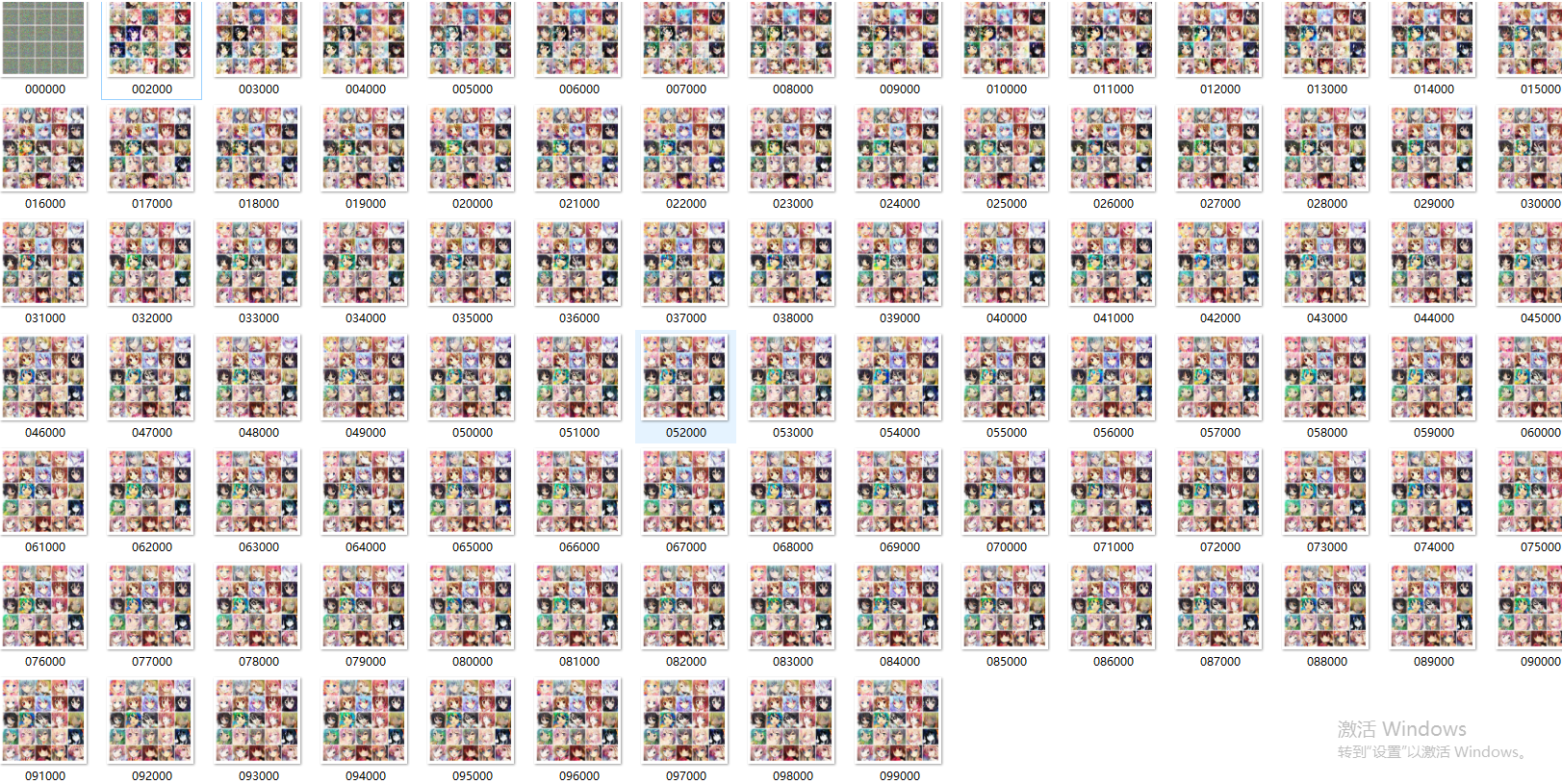
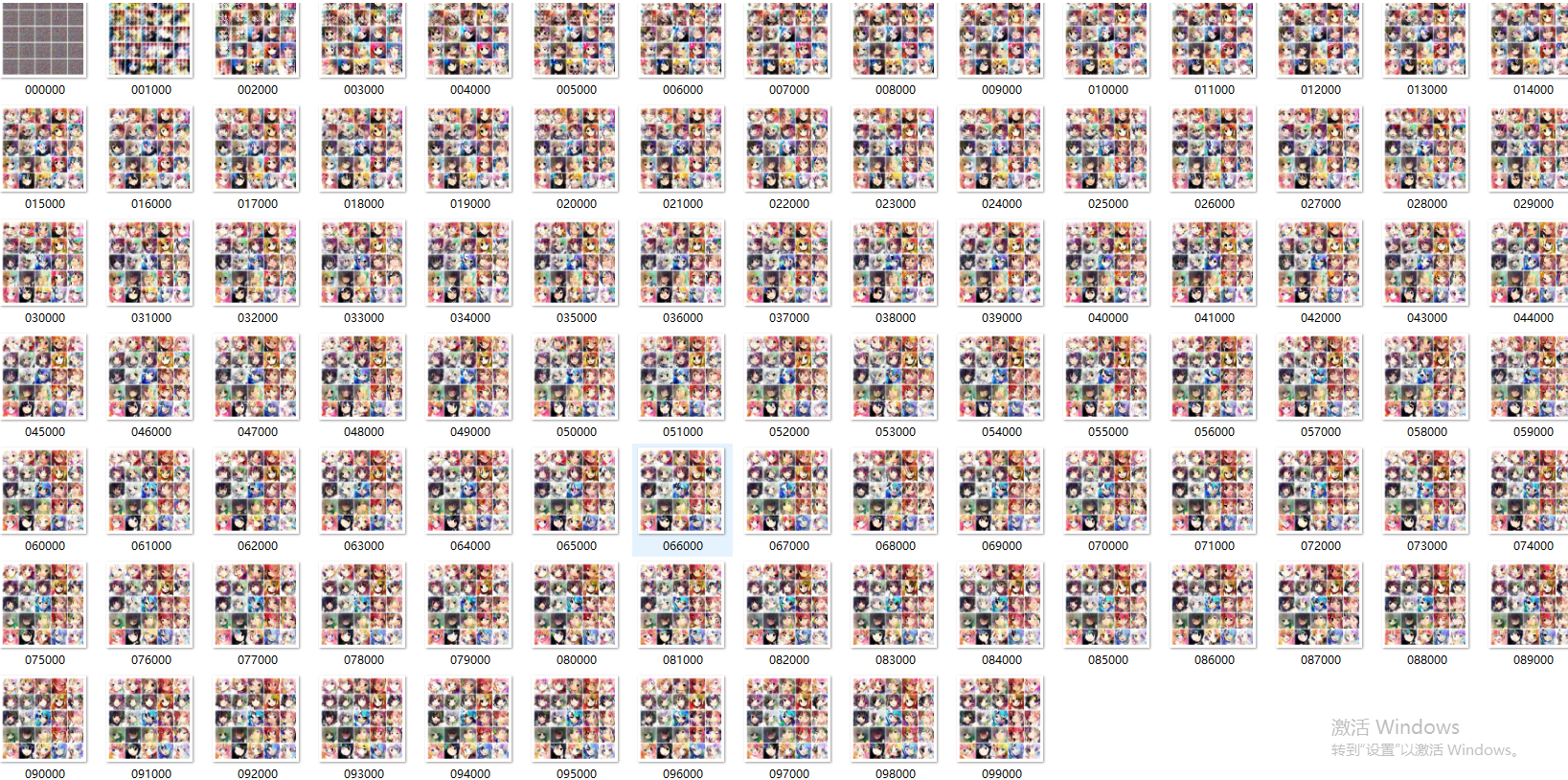
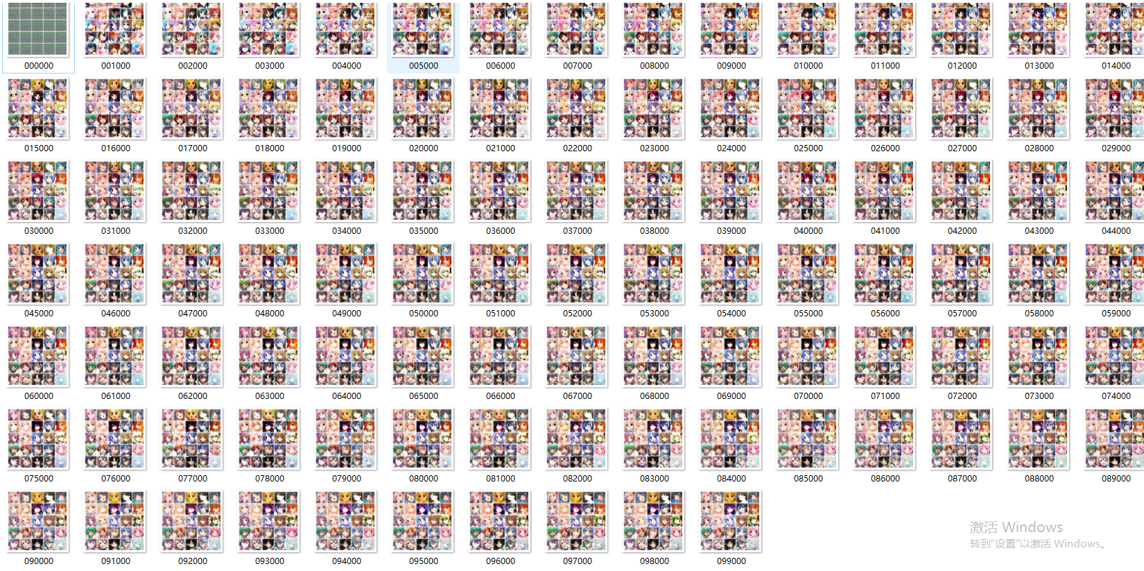
Training results

LSGAN

WGAN

WGAN—GP

summary

1.LSGAN does not use Sigmoid activation function, and uses linear activation function instead of Sigmoid activation function for linear regression.
2.WGAN cuts the weight and sets the cutting range according to the constraint conditions.
3.WGAN-GP averages the real data and generated data and sends them to the discriminator to calculate the gradient constraint.
4.EBGAN is to use the automatic encoder instead of the discriminator to train and reconstruct the real picture in advance.
5.WGAN-GP has the best effect, but the training time is relatively long.

reference

[1] I. Goodfellow, J. Pouget-Abadie, M. Mirza, B. Xu, D. Warde-Farley,
S. Ozair, A. Courville, and Y. Bengio, "Generative adversarial nets," in Advances in Neural Information Processing Systems (NIPS), pp. 2672–2680,2014.
[2] T. Salimans, I. Goodfellow, W. Zaremba, V. Cheung, A. Radford, X. Chen,
and X. Chen, "Improved techniques for training gans," in Advances in
Neural Information Processing Systems (NIPS), pp. 2226–2234, 2016.
[3]M. Arjovsky, S. Chintala, and L. Bottou, "Wasserstein gan,"
arXiv:1701.07875, 2017.

other

This paper is an improvement of training skills based on GAN and DCGAN. LSGAN, WGAN, WGAN-GP and EBGAN all improve the training skills in different places and get a better training effect.
Article code: link: https://pan.baidu.com/s/14No7ikUIbH2MvNp3DyNbLA
Extraction code: q5ol