Source: ICML2019

Paper link: https://arxiv.org/abs/1901.09590

Code link: https://github.com/ibalazevic/TuckER

• Conclusion: This article uses an advanced formula. Many people may be afraid when they see this formula. Indeed, I feel dizzy when I see this formula and don't know the specific meaning. In fact, if you really don't understand the specific meaning, you can ignore it and roughly understand the author's idea. I read the code after reading the paper, So I have a certain understanding of the training process of this article, and then read the paper again. You can also use this learning method to read paper.

1. Background knowledge

1.1 Tucker Decomposition

• Definition: decompose a tensor into a set of matrices and a core tensor

• The formula is as follows:
  X ≈ Z × 1 A × 2 B × 3 C \mathcal{X} \approx \mathcal{Z} \times_{1} \mathbf{A} \times{ }_{2} \mathbf{B} \times{ }_{3} \mathbf{C} X≈Z×1​A×2​B×3​C
  Of which: X ∈ R I × J × K \mathcal{X} \in \mathbb{R}^{I \times J \times K } X∈RI×J×K, Z ∈ R P × Q × R \mathcal{Z} \in \mathbb{R}^{P \times Q \times R} Z∈RP×Q×R, A ∈ R I × P A \in \mathbb{R}^{I \times P} A∈RI×P, B ∈ R J × Q B \in \mathbb{R}^{J \times Q} B∈RJ×Q, C ∈ R K × R C \in \mathbb{R}^{K \times R} C∈RK×R

• Formula interpretation:

  • × n \times_{n} × N ＾ represents the tensor product along mode n (which can be simply understood as a simplified formulation of the calculation formula)
  • A. B and C can be understood as the principal components in each mode.
  • Z \mathcal{Z} Each element in Z represents the degree of interaction between different components.
  • Where P, Q and R are less than I, J and K respectively, so it can also be considered that Z \mathcal{Z} Z is X \mathcal{X} Compressed version of X

2. Model architecture

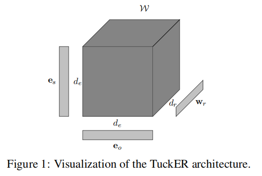
• Scoring function:
  ϕ ( e s , r , e o ) = W × 1 e s × 2 w r × 3 e o \phi\left(e_{s}, r, e_{o}\right)=\mathcal{W} \times_{1} \mathbf{e}_{s} \times_{2} \mathbf{w}_{r} \times_{3} \mathbf{e}_{o} ϕ(es​,r,eo​)=W×1​es​×2​wr​×3​eo​
  Of which: e s , w r , e o \mathbf{e}_{s},\mathbf{w}_{r},\mathbf{e}_{o} es, wr and eo denote the embedding of head entity, relation and tail entity; d e , d r d_e,d_r de and dr represent the embedded dimensions of entities and relationships respectively; W ∈ R d e × w r × d e \mathcal{W} \in \mathbb{R}^{d_e \times w_r \times d_e} W∈Rde​ × wr​ × de = kernel tensor

3. Model training

• Input the result obtained from the above scoring function into the sigmoid function to obtain a probability value, and then calculate the following loss value:
  L = − 1 n e ∑ i = 1 n e ( y ( i ) log ⁡ ( p ( i ) ) + ( 1 − y ( i ) ) log ⁡ ( 1 − p ( i ) ) ) L=-\frac{1}{n_{e}} \sum_{i=1}^{n_{e}}\left(\mathbf{y}^{(i)} \log \left(\mathbf{p}^{(i)}\right)+\left(1-\mathbf{y}^{(i)}\right) \log \left(1-\mathbf{p}^{(i)}\right)\right) L=−ne​1​i=1∑ne​​(y(i)log(p(i))+(1−y(i))log(1−p(i)))
  Where: when the triples are correct, y=1; otherwise, y=0

• Before looking at the code, I think this scoring function is to score the whole triplet. In fact, it doesn't mean that in the code

• The output of forward propagation calculation is a matrix with the size of (batch,len(entity)), and the input is the head entity and relationship of a batch, which is equivalent to the probability value of the occurrence of the tail entity at each position in the prediction. Then, the matrix composed of this probability value and the target position (the correct position is 1) is used to calculate the loss (which can be understood as a binary classification problem)

4. Core code and explanation

class TuckER(torch.nn.Module):
    def __init__(self, d, d1, d2, **kwargs):
        '''
        :param d: data set
        :param d1: Entity embedded dimension 200
        :param d2: Relationship embedding dimension 200
        :param kwargs: Dictionaries
        '''
        super(TuckER, self).__init__()
        self.E = torch.nn.Embedding(len(d.entities), d1)
        self.R = torch.nn.Embedding(len(d.relations), d2)
        self.W = torch.nn.Parameter(torch.tensor(np.random.uniform(-1, 1, (d2, d1, d1)),
                                                 dtype=torch.float, device="cuda", requires_grad=True))
        self.input_dropout = torch.nn.Dropout(kwargs["input_dropout"])
        self.hidden_dropout1 = torch.nn.Dropout(kwargs["hidden_dropout1"])
        self.hidden_dropout2 = torch.nn.Dropout(kwargs["hidden_dropout2"])
        self.loss = torch.nn.BCELoss()	# Cross entropy loss similar to binary classification
        self.bn0 = torch.nn.BatchNorm1d(d1)
        self.bn1 = torch.nn.BatchNorm1d(d1)
        torch.nn.init.xavier_normal_(self.E.weight.data)
        torch.nn.init.xavier_normal_(self.R.weight.data)

    def forward(self, e1_idx, r_idx):
        '''Simple understanding: pred=e1*r*W*E'''
        e1 = self.E(e1_idx)
        x = self.bn0(e1)
        x = self.input_dropout(x)  # [128,200]
        x = x.view(-1, 1, e1.size(1))  # [128,1,200]
		
        r = self.R(r_idx)
        W_mat = torch.mm(r, self.W.view(r.size(1), -1))  # [128,40000]
        W_mat = W_mat.view(-1, e1.size(1), e1.size(1))  # [128,200,200]
        W_mat = self.hidden_dropout1(W_mat)

        x = torch.bmm(x, W_mat)  # [128,1,200]
        x = x.view(-1, e1.size(1))  # [128,200]
        x = self.bn1(x)
        x = self.hidden_dropout2(x)
        x = torch.mm(x, self.E.weight.transpose(1, 0))  # Transfer is equivalent to transpose [12814541]
        pred = torch.sigmoid(x)
        return pred

• Model analysis:

  • There are 13 parameters to be trained in this model

    W
    E.weight
    R.weight
    bn0.weight
    bn0.bias
    bn0.running_mean
    bn0.running_var
    bn0.num_batches_tracked
    bn1.weight
    bn1.bias
    bn1.running_mean
    bn1.running_var
    bn1.num_batches_tracked
    

  • In the training process, anti relational triples are added