1. Spark SQL architecture design
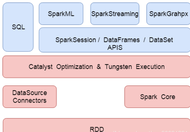
The development of big data is realized by using SQL directly. It supports both DSL and SQL syntax style. At present, in the whole architecture design of spark, all spark modules, such as SQL, SparkML, sparkGrahpx and structured streaming, run on the catalyst optimization & tungsten execution module, The following figure shows the overall architecture and module design of spark
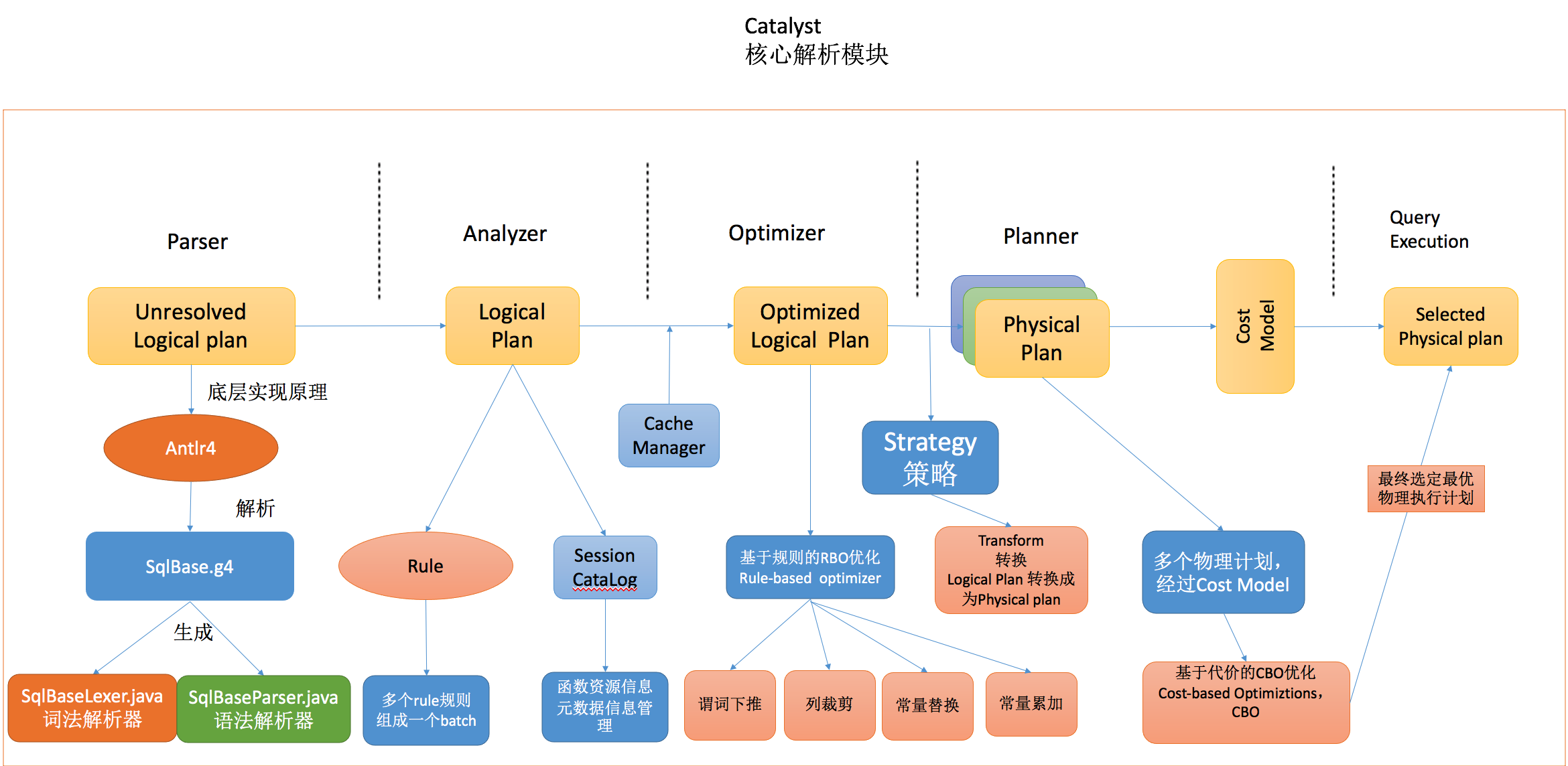
2. SparkSQL execution process
- Parser: use Antlr4 to parse the morphology and syntax of sql statements
- Analyzer: it mainly uses the Catalog information to parse the Unresolved Logical Plan into the Analyzed logical plan;
- Optimizer: use some rules to resolve the Analyzed logical plan into Optimized Logical Plan;
- Planner: the previous logical plan cannot be executed by Spark. This process is to convert the logical plan into multiple physical plans, and then use the cost model to select the best physical plan;
- Code Generation: this process will generate Java bytecode from SQL query.
3. SQL example
For example, execute the following SQL statement:
select temp1.class,sum(temp1.degree),avg(temp1.degree) from (SELECT students.sno AS ssno,students.sname,students.ssex,students.sbirthday,students.class, scores.sno,scores.degree,scores.cno FROM students LEFT JOIN scores ON students.sno = scores.sno ) temp1 group by temp1.class
The code implementation process is as follows:
package com.kkb.sparksql
import java.util.Properties
import org.apache.spark.SparkConf
import org.apache.spark.sql.{DataFrame, SparkSession}

//todo: using sparksql to load data in mysql tables
object DataFromMysqlPlan {
  def main(args: Array[String]): Unit = {
    //1. Create a SparkConf object
    val sparkConf: SparkConf = new SparkConf().setAppName("DataFromMysql").setMaster("local[2]")

    //sparkConf.set("spark.sql.codegen.wholeStage","true")
    //2. Create a SparkSession object
    val spark: SparkSession = SparkSession.builder().config(sparkConf).getOrCreate()
    spark.sparkContext.setLogLevel("WARN")

    //3. Read data from mysql table
    //3.1 specify mysql connection address
    val url="jdbc:mysql://localhost:3306/mydb?characterEncoding=UTF-8"
    //3.2 specify the table name to load
    val student="students"
    val score="scores"

    // 3.3 configure the related attributes of the connection database
    val properties = new Properties()

    //user name
    properties.setProperty("user","root")
    //password
    properties.setProperty("password","123456")

    val studentFrame: DataFrame = spark.read.jdbc(url,student,properties)
    val scoreFrame: DataFrame = spark.read.jdbc(url,score,properties)
    //Register dataFrame as a table
    studentFrame.createTempView("students")
    scoreFrame.createOrReplaceTempView("scores")
    //spark.sql("SELECT temp1.class,SUM(temp1.degree),AVG(temp1.degree) FROM (SELECT  students.sno AS ssno,students.sname,students.ssex,students.sbirthday,students.class, scores.sno,scores.degree,scores.cno  FROM students LEFT JOIN scores ON students.sno =  scores.sno ) temp1  GROUP BY temp1.class; ").show()
    val resultFrame: DataFrame = spark.sql("SELECT temp1.class,SUM(temp1.degree),AVG(temp1.degree)  FROM (SELECT  students.sno AS ssno,students.sname,students.ssex,students.sbirthday,students.class, scores.sno,scores.degree,scores.cno  FROM students LEFT JOIN scores ON students.sno =  scores.sno  WHERE degree > 60 AND sbirthday > '1973-01-01 00:00:00' ) temp1 GROUP BY temp1.class")
    resultFrame.explain(true)
    resultFrame.show()
    spark.stop()
  }
}
4. Catalyst execution process
From the above query plan, we can see that the sql statement we write is finally compiled into a bytecode file for execution after multiple transformations (note that the figure is viewed from bottom to top), including the following important steps
- parse in sql parsing phase
- Generate logical plan Analyzer
- sql statement tuning phase Optimizer
- Generate physical query plan planner
4.1 sql parsing phase Parser
Antlr is used in our common big data SQL parsing, including Hive, Cassandra, Phoenix, Pig and presto. It can read, process, execute and translate structured text or binary files. It is the most widely used syntax generator tool in the current Java language.
At present, the latest version of spark uses antlr4, which is used for lexical analysis of SQL and construction of syntax tree. We can check the source code of spark through github
If you need to reconstruct the syntax of sparkSQL, use sqlbase G4 performs syntax parsing and generates relevant java classes, including
- Lexical parser sqlbaselexer java
- Syntax parser sqlbaseparser java.
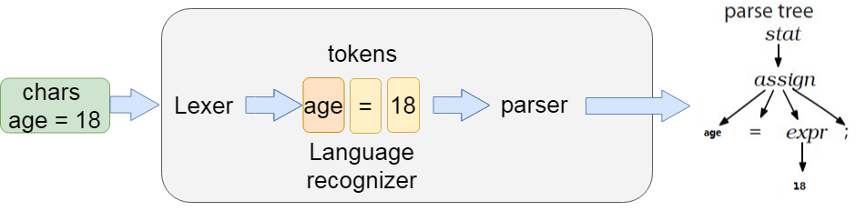
Finally, after parsing through Lexer and parse, generate the syntax tree. After generating the syntax tree, use AstBuilder to convert the syntax tree into LogicalPlan, which is also called Unresolved LogicalPlan.
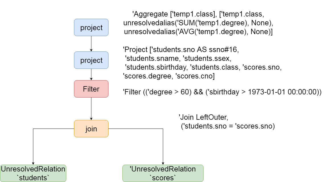
The logic plan after parsing is as follows:,
== Parsed Logical Plan ==
'Aggregate ['temp1.class], ['temp1.class, unresolvedalias('SUM('temp1.degree), None), unresolvedalias('AVG('temp1.degree), None)]
+- 'SubqueryAlias temp1
   +- 'Project ['students.sno AS ssno#16, 'students.sname, 'students.ssex, 'students.sbirthday, 'students.class, 'scores.sno, 'scores.degree, 'scores.cno]
      +- 'Filter (('degree > 60) && ('sbirthday > 1973-01-01 00:00:00))
         +- 'Join LeftOuter, ('students.sno = 'scores.sno)
            :- 'UnresolvedRelation `students`
            +- 'UnresolvedRelation `scores`

As can be seen from the above figure, after the two tables are join ed, an unresolved relation is generated. The selected columns and aggregated fields are available. The first stage of sql parsing has been completed, and then it is ready to enter the second stage
4.2 binding logical plan Analyzer
In the parse phase of sql parsing, many unresolved keywords are generated, which are part of the Unresolved LogicalPlan parsing. Unresolved LogicalPlan is just a data structure and does not contain any data information. For example, you do not know the data source, data type, which table different columns come from, and so on..
The Analyzer phase will use the pre-defined rules, SessionCatalog and other information to transform the Unresolved LogicalPlan. SessionCatalog is mainly used for the unified management of various function resource information and metadata information (database, data table, data view, data partition and function, etc.). The Rule is defined in Analyzer, and the specific class path is as follows
org.apache.spark.sql.catalyst.analysis.Analyzer

concrete rule The rules are defined as follows:
 lazy val batches: Seq[Batch] = Seq(
    Batch("Hints", fixedPoint,
      new ResolveHints.ResolveBroadcastHints(conf),
      ResolveHints.RemoveAllHints),
    Batch("Simple Sanity Check", Once,
      LookupFunctions),
    Batch("Substitution", fixedPoint,
      CTESubstitution,
      WindowsSubstitution,
      EliminateUnions,
      new SubstituteUnresolvedOrdinals(conf)),
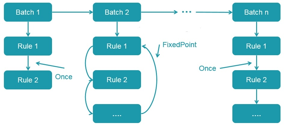
Multiple rules with similar properties form a Batch, while multiple batches form a Batch. These batches will be executed by the RuleExecutor, first in Batch order, and then in order for each Rule in the Batch. Each Batch will execute Once or multiple times (FixedPoint, determined by spark.sql.optimizer.maxIterations parameter). The execution process is as follows:
-
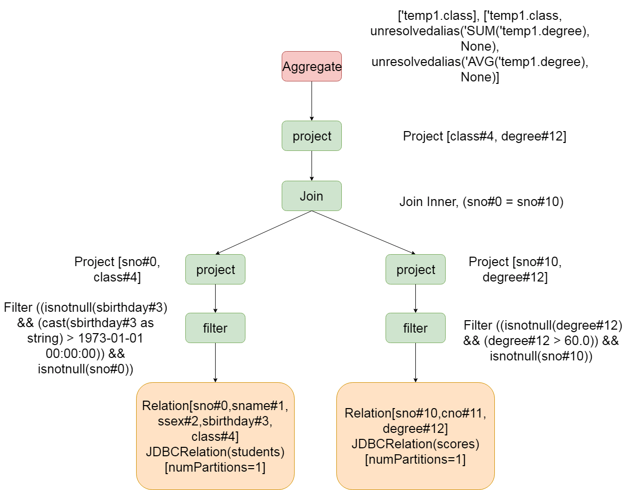
Therefore, the Analyzed Logical Plan generated by the above SQL at this stage is as follows:
== Analyzed Logical Plan ==
class: string, sum(degree): decimal(20,1), avg(degree): decimal(14,5)
Aggregate [class#4], [class#4, sum(degree#12) AS sum(degree)#27, avg(degree#12) AS avg(degree)#28]
+- SubqueryAlias temp1
   +- Project [sno#0 AS ssno#16, sname#1, ssex#2, sbirthday#3, class#4, sno#10, degree#12, cno#11]
      +- Filter ((cast(degree#12 as decimal(10,1)) > cast(cast(60 as decimal(2,0)) as decimal(10,1))) && (cast(sbirthday#3 as string) > 1973-01-01 00:00:00))
         +- Join LeftOuter, (sno#0 = sno#10)
            :- SubqueryAlias students
            :  +- Relation[sno#0,sname#1,ssex#2,sbirthday#3,class#4] JDBCRelation(students) [numPartitions=1]
            +- SubqueryAlias scores
               +- Relation[sno#10,cno#11,degree#12] JDBCRelation(scores) [numPartitions=1]
From the above parsing process, the students and scores tables have been parsed into specific fields, including aggregate functions. The types of the four fields finally returned have also been determined, and it is also known that the data sources are JDBC relation (students) table and JDBC relation (scores) table.
In conclusion, the Analyzed Logical Plan has mainly done some of these things
1. Determine the final return field name and return type:
2. Determine aggregate function
3. Determine the query fields obtained in the table
4. Determine filter conditions
5. Determine the join method
6. Determine the data source and the number of partitions in the table
4.3 logic optimization phase Optimizer
The optimizer at this stage is mainly Rule-based Optimizer (RBO), and most of the rules are heuristic rules, that is, rules based on intuition or experience
Similar to the binding logic plan phase described earlier, all rules in this phase also implement the Rule abstract class. Multiple rules form a Batch and multiple batches form a Batch. They are also executed in the RuleExecutor. Here, they are explained one by one according to the Rule execution order.
4.3.1 predicate push down
Predicate pushdown is implemented by PushDownPredicate in SparkQL. This process mainly pushes the filter conditions to the bottom as much as possible, preferably the data source.
As shown in the figure, predicate push down pushes the Filter operator directly before the Join, that is, when scanning the student table, use conditional filtering conditions to Filter the data that meets the conditions; At the same time, when scanning the t2 table, the data meeting the conditions will be filtered by using the isnotnull (id#8) & & (id#8 > 50000) Filter conditions. After such operation, the amount of data processed by the Join operator can be greatly reduced, so as to speed up the calculation speed
4.3.2 column clipping
Column clipping is implemented by ColumnPruning in Spark SQL. The use of column clipping can filter out the fields that are not needed by the query, so as to reduce the amount of scanned data.
After column clipping, the students table only needs to query sno and class fields; The scores table only needs to query the sno and degree fields. This reduces the transmission of data, and if the underlying file format is column storage (such as Parquet), it can greatly improve the scanning speed of data.
4.3.3 constant substitution
Constant substitution is implemented by ConstantPropagation in Spark SQL. That is, replace variables with constants,
SELECT * FROM table WHERE i = 5 AND j = i + 3 can be converted to SELECT * FROM table WHERE i = 5 AND j = 8.
4.3.4 constant accumulation
-
Constant accumulation in Spark SQL is realized by constant folding. This is similar to constant substitution. It is also at this stage that some constant expressions are calculated in advance.
-
Therefore, after the optimization of the above four steps, the optimized logical plan is
== Optimized Logical Plan ==
Aggregate [class#4], [class#4, sum(degree#12) AS sum(degree)#27, cast((avg(UnscaledValue(degree#12)) / 10.0) as decimal(14,5)) AS avg(degree)#28]
+- Project [class#4, degree#12]
   +- Join Inner, (sno#0 = sno#10)
      :- Project [sno#0, class#4]
      :  +- Filter ((isnotnull(sbirthday#3) && (cast(sbirthday#3 as string) > 1973-01-01 00:00:00)) && isnotnull(sno#0))
      :     +- Relation[sno#0,sname#1,ssex#2,sbirthday#3,class#4] JDBCRelation(students) [numPartitions=1]
      +- Project [sno#10, degree#12]
         +- Filter ((isnotnull(degree#12) && (degree#12 > 60.0)) && isnotnull(sno#10))
            +- Relation[sno#10,cno#11,degree#12] JDBCRelation(scores) [numPartitions=1]
- So far, the optimization logic stage has been basically completed. For more other optimizations, see spark's optimizer scala Source code
4.4 generate executable Physical Plan
After a series of policy processing, a Logical Plan obtains multiple Physical Plans, which are implemented by SparkPlan in Spark. Multiple Physical Plans are selected through the Cost Model. The whole process is as follows: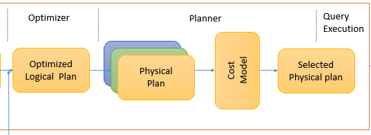
Cost Model corresponds to cost based optimizations (CBO), which is mainly implemented by Huawei bosses. See SPARK-16026 for details). The core idea is to calculate the cost of each physical plan and then obtain the optimal physical plan. However, in the latest version of Spark 2.4.3, this part is not implemented. The first of multiple physical plan lists is directly returned as the optimal physical plan
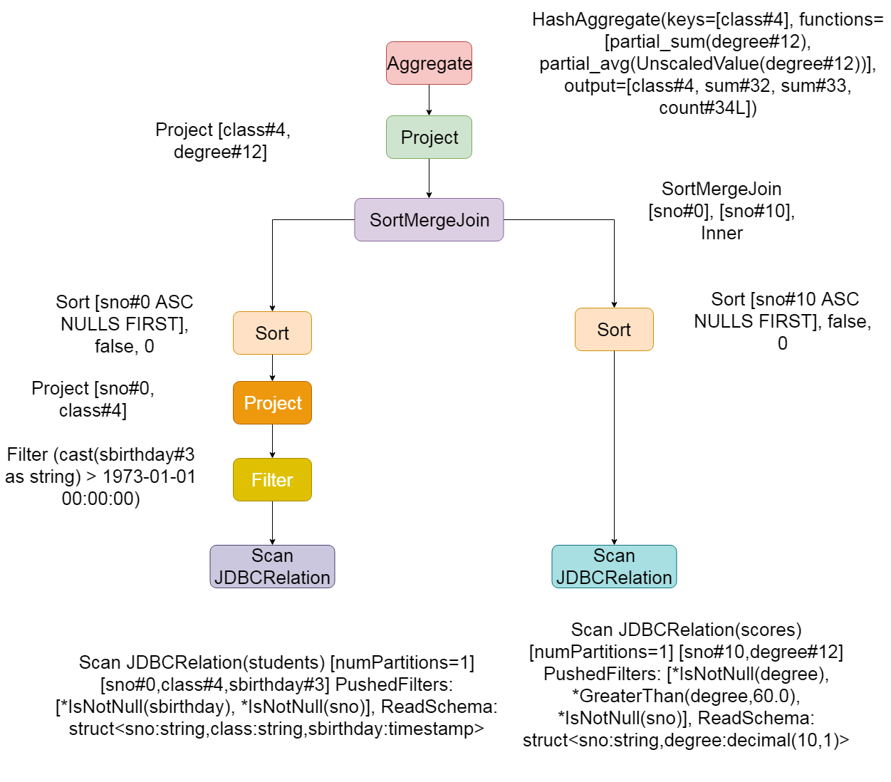
== Physical Plan ==
*(6) HashAggregate(keys=[class#4], functions=[sum(degree#12), avg(UnscaledValue(degree#12))], output=[class#4, sum(degree)#27, avg(degree)#28])
+- Exchange hashpartitioning(class#4, 200)
   +- *(5) HashAggregate(keys=[class#4], functions=[partial_sum(degree#12), partial_avg(UnscaledValue(degree#12))], output=[class#4, sum#32, sum#33, count#34L])
      +- *(5) Project [class#4, degree#12]
         +- *(5) SortMergeJoin [sno#0], [sno#10], Inner
            :- *(2) Sort [sno#0 ASC NULLS FIRST], false, 0
            :  +- Exchange hashpartitioning(sno#0, 200)
            :     +- *(1) Project [sno#0, class#4]
            :        +- *(1) Filter (cast(sbirthday#3 as string) > 1973-01-01 00:00:00)
            :           +- *(1) Scan JDBCRelation(students) [numPartitions=1] [sno#0,class#4,sbirthday#3] PushedFilters: [*IsNotNull(sbirthday), *IsNotNull(sno)], ReadSchema: struct<sno:string,class:string,sbirthday:timestamp>
            +- *(4) Sort [sno#10 ASC NULLS FIRST], false, 0
               +- Exchange hashpartitioning(sno#10, 200)
                  +- *(3) Scan JDBCRelation(scores) [numPartitions=1] [sno#10,degree#12] PushedFilters: [*IsNotNull(degree), *GreaterThan(degree,60.0), *IsNotNull(sno)], ReadSchema: struct<sno:string,degree:decimal(10,1)>
- From the above results, it can be seen that the physical planning stage already knows that the data source is read from JDBC, as well as the path and data type of the file. Moreover, when reading the file, the pushed filters are directly added. At the same time, the Join becomes sortmerge Join,
4.5 code generation phase
After the execution of the above processes, we finally get the physical execution plan, which indicates the whole code execution process
- Execution process
- Data fields and field types,
- Location of data source
However, the physical execution plan is obtained, but if the physical execution plan wants to be executed, it still needs to generate complete code, and the bottom layer is processed based on sparkRDD
4.5.1 difference between generated code and sql parsing engine
- In spark sql, the final generation of sql statements is realized by generating code. To put it bluntly, the bottom layer is still executing code. However, in spark 2 Before version 0, it was based on the Volvo iterator model (see the Volvo an extensible and parallel query evaluation system)
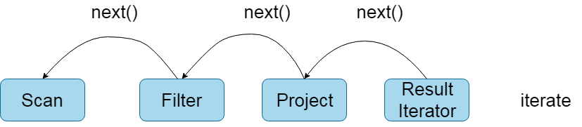
- Most of today's database systems deal with SQL based on this model at the bottom. The implementation of this model can be summarized as follows: first, the database engine will translate SQL into a series of relational algebra operators or expressions, and then rely on these relational algebra operators to process the input data one by one and produce results. Each operator implements the same interface at the bottom layer. For example, it implements the next() method, and then the operator next() at the top layer calls the next() of the sub operator, and the next() of the sub operator calls the next() of the sub operator until the next() at the bottom layer. The specific process is shown in the following figure:
- The advantage of Volvo iterator model is that it is very simple to abstract and easy to implement, and complex queries can be expressed by any combination operator. However, the disadvantages are also obvious. There are a large number of virtual function calls, which will cause CPU interruption and ultimately affect the execution efficiency. The official blog of databricks has compared the execution efficiency of using Volcano Iterator Model and handwritten code, and found that the execution efficiency of handwritten code is ten times higher! So to sum up, parsing sql into code is faster than parsing sql statements directly by sql Engine, so spark 2 0 finally chose to use code generation to execute sql statements
4.5.2 Tungsten code generation is divided into three parts:
- expression codegen
- Whole stage code generation
- speed up serialization/deserialization
Expression code generation
This is actually in spark 1 X is there. The base class generated by the expression code is org apache. spark. sql. catalyst. expressions. codegen. Codegenerator, which has seven subclasses:
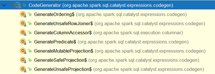
(is not null (sbirthday #3) & & (cast (sbirthday #3 as string) > 1973-01-01 00:00:00) in the logic plan generated by SQL is the most basic expression. It is also a Predicate, so it will call org apache. spark. sql. catalyst. expressions. codegen. Generate predict to generate the code of the expression. Expression code generation mainly aims to solve a large number of Virtual Function Calls and the cost of generalization
Whole stage code generation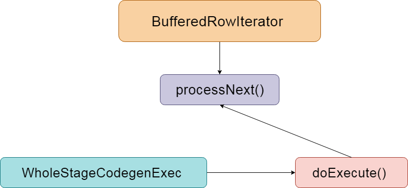
Whole stage code generation is used to integrate multiple processing logic into a single code module, in which the above expression code generation is also used. Unlike the expression code generation described earlier, this is to generate the code of the whole SQL process. The previous expression code generation is only for the expression.
Compared with the Volvo iterator model, the execution process of full-stage code generation is as follows: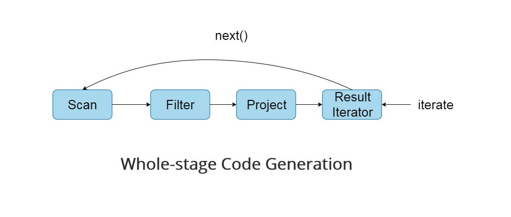
By introducing full-stage code generation, the calls of virtual functions and CPU are greatly reduced, which greatly improves the execution speed of SQL.
Code compilation
Code generation is carried out on the Driver side, while code compilation is carried out on the Executor side.
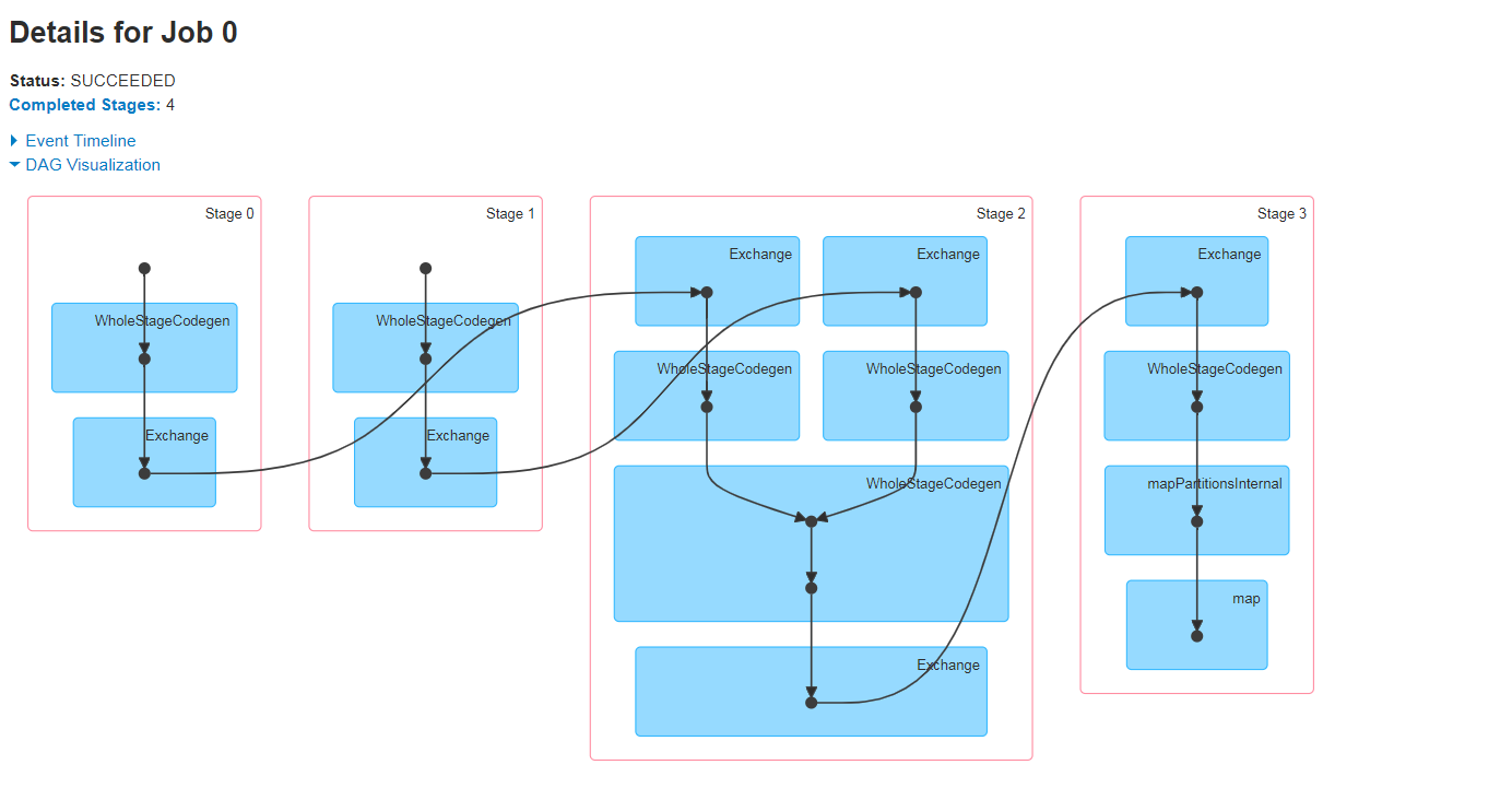
SQL execution
Finally, it's the place where SQL is really executed. At this time, Spark will execute the code generated in the previous stage and get the final result. The DAG execution diagram is as follows:
5. Spark SQL execution process summary

Main steps:
Enter sql, dataFrame or dataSet
After the Catalyst process, the optimal physical execution plan is generated
parser phase
It is mainly used to parse sqlbase.xml through Antlr4 G4, all syntax supported by spark are defined in sqlbase In G4, we generated our syntax parser sqlbaselexer Java and lexical parser sqlbaseparser java
Parse phase -- > antlr4 - > parse - > sqlbase G4 - > syntax parser sqlbaselexer Java + lexical parser sqlbaseparser java
analyzer phase
Use Rule-based Rule parsing and Session Catalog to realize function resource information and metadata management information
Analyzer stage -- > use -- > rule + session catalog -- > multiple rules -- > to form a batch -- > session catalog -- > to save function resource information and metadata information
optimizer phase
Optimizer tuning stage -- > rule-based optimization of RBO rule-based optimizer -- > predicate push down + column pruning + constant replacement + constant accumulation
planner stage
Generate multiple physical plans -- > make optimal selection through Cost Model -- > CBO optimization based on cost -- > finally select the optimal physical execution plan
Select the final physical plan and prepare for execution
Finally, the selected optimal physical execution plan -- > is ready to generate code to start execution
Generate the final physical execution plan and submit the code to perform our final task