The content of this article comes from learning MIT open course: univariate calculus - definite integral - Netease open course

1, Concept of definite integral

Cumulative area (under other geometry)

​

 

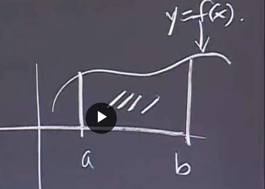
The difference between an indefinite integral and an indefinite integral is that an indefinite integral does not give an upper or lower limit (a,b)

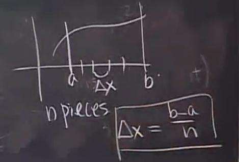
2, To calculate an area

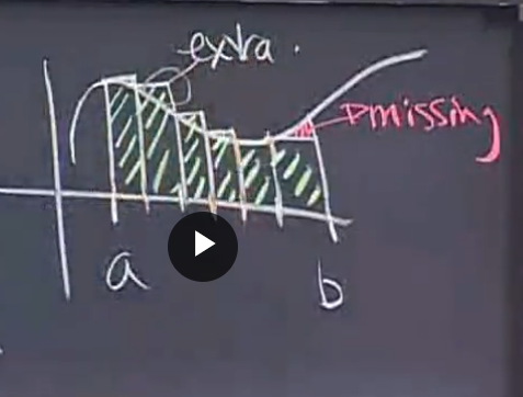
1. Cut into multiple "rectangles"

2. Add up the areas of these "rectangles"

3. Correct the previous result (get the limit value by narrowing the "Rectangle" to infinity)

​

 

3, Examples

1, , a = 0, b any

Area=

Here's the calculation , the teacher gave an algorithm to treat each number in the sequence as an edge of the lower bottom surface (square) of a cuboid with a height of 1, thus forming a pyramid. In addition, the pyramid has an internal 4-pyramid and an external 4-pyramid.

The volume is

import matplotlib as mpl
from matplotlib import cm
from matplotlib import pyplot as plt
from mpl_toolkits.mplot3d.art3d import Poly3DCollection, Line3DCollection
from mpl_toolkits.mplot3d import Axes3D
# Create canvas
fig = plt.figure(figsize=(12, 8),
                 facecolor='lightyellow'
                )

# Create 3D coordinate system
ax = fig.gca(fc='whitesmoke',
               projection='3d' 
              )


# Draw 3D graphics

ax.plot3D(xs=[5, 0, 0, 0, 0, ],    # x-axis coordinates
          ys=[0, 0, 5, 0, 0, ],    # y-axis coordinates
          zs=[0, 0, 0, 0, 5, ],    # z-axis coordinates
          zdir='z',    # 
          c='k',    # color
          marker='o',    # Mark point symbol
          mfc='r',    # marker facecolor
          mec='g',    # marker edgecolor
          ms=10,    # size
        )


def plot_opaque_cube(x, y, z, dx, dy, dz, ax):

    xx = np.linspace(x, x+dx, 2)
    yy = np.linspace(y, y+dy, 2)
    zz = np.linspace(z, z+dz, 2)

    xx, yy = np.meshgrid(xx, yy)

    
    #ax.plot_surface(xx, yy, z)
    #ax.plot_surface(xx, yy, z+dz)

    yy, zz = np.meshgrid(yy, zz)
    ax.plot_surface(x, yy, zz)
    ax.plot_surface(x+dx, yy, zz)

    xx, zz = np.meshgrid(xx, zz)
    ax.plot_surface(xx, y, zz)
    ax.plot_surface(xx, y+dy, zz)
    # ax.set_xlim3d(-dx, dx*2, 20)
    # ax.set_xlim3d(-dx, dx*2, 20)
    # ax.set_xlim3d(-dx, dx*2, 20)

def drawPyramid(height,steps, ax, printTitle):
    zFrom = 0
    V = 0
    for step in range(steps):
        width = steps-step
        plot_opaque_cube(0 - width/2, 0 - width/2, zFrom, width,width,height, ax)
        V += width * width * height
        zFrom += height
    print(printTitle + ' = ', V)
        

def drawPyramid1(height,steps,ax, edgecolor, printTitle):
    # vertices of a pyramid
    width = steps - 0
    
    v = np.array([[0-width/2, 0-width/2, 0], [width/2, 0-width/2, 0], [width/2, width/2, 0],  [0-width/2, width/2, 0], [0, 0, height* steps]])
    
    ax.scatter3D(v[:, 0], v[:, 1], v[:, 2])

    # generate list of sides' polygons of our pyramid
    verts = [ [v[0],v[1],v[4]], [v[0],v[3],v[4]],
     [v[2],v[1],v[4]], [v[2],v[3],v[4]], [v[0],v[1],v[2],v[3]]]

    # plot sides
    ax.add_collection3d(Poly3DCollection(verts, 
     facecolors='gray', linewidths=1, edgecolors=edgecolor, alpha=.25))        
    
    V = width * width * height* steps / 3
    print(printTitle + ' = ', V)

# Adjust Perspective
ax.view_init(elev=20,    # elevation
             azim=40    # azimuth
            )

drawPyramid1(1,10, ax, 'r', 'n*n*n/3')
drawPyramid(1, 10, ax, '1 + 2*2 + ... + n*n')
drawPyramid1(1,11, ax, 'g', '(n+1)*(n+1)*(n+1)')
# display graphics
plt.show()

​

 

Follow the above formula:

Area= (the focus here is to consider that the volume of an infinite layered pyramid is equivalent to the volume of a 4-pyramid, so the cumulative term can be simplified)

Inequality:

So area:

=

Here the teacher introduced the summation symbol

Area:

2. F (x) = x, a = 0, B arbitrary

from sympy import *
import numpy as np 

import matplotlib.pyplot as plt 

fig = plt.figure()
ax = fig.add_subplot(1, 1, 1)
ax.spines['left'].set_position('zero')
ax.spines['bottom'].set_position('zero')
ax.spines['right'].set_color('none')
ax.spines['top'].set_color('none')
ax.xaxis.set_ticks_position('bottom')
ax.yaxis.set_ticks_position('left')
ax.set_aspect(1 ) 

def DrawXY(xFrom,xTo,steps,expr,color,label,plt):
    yarr = []
    xarr = np.linspace(xFrom ,xTo, steps) 
    for xval in xarr:
        yval = expr.subs(x,xval)
        yarr.append(yval)
    y_nparr = np.array(yarr) 
    plt.plot(xarr, y_nparr, c=color, label=label)    

def DrawRects(xFrom,xTo,steps,expr,color,plt):
    width = (xTo - xFrom)/steps
    xarrRect = []
    yarrRect = []
    area = 0
    xprev = xFrom
    for step in range(steps):
        yval = expr.subs(x,xprev + width)
        xarrRect.append(xprev)
        xarrRect.append(xprev)
        xarrRect.append(xprev + width)
        xarrRect.append(xprev + width)
        xarrRect.append(xprev)
        yarrRect.append(0)
        yarrRect.append(yval)
        yarrRect.append(yval)
        yarrRect.append(0)
        yarrRect.append(0)
        area += width * yval
        plt.plot(xarrRect, yarrRect, c=color)    
        xprev= xprev + width
    print('width =', width)
    print('area=',area)

def TangentLine(exprY,x0Val,xVal):
    diffExpr = diff(exprY)
    x1,y1,xo,yo = symbols('x1 y1 xo yo')
    expr = (y1-yo)/(x1-xo) - diffExpr.subs(x,x0Val)
    eq = expr.subs(xo,x0Val).subs(x1,xVal).subs(yo,exprY.subs(x,x0Val))
    eq1 = Eq(eq,0)
    solveY = solve(eq1)
    return xVal,solveY

def DrawTangentLine(exprY, x0Val,xVal1, xVal2, clr, txt):
    x1,y1 = TangentLine(exprY, x0Val, xVal1)
    x2,y2 = TangentLine(exprY, x0Val, xVal2)
    plt.plot([x1,x2],[y1,y2], color = clr, label=txt)
    
def Newton(expr, x0):
    ret = x0 - expr.subs(x, x0)/ expr.diff().subs(x,x0)
    return ret

x = symbols('x')
expr = x

DrawXY(0,5,100,expr,'blue','',plt)
DrawRects(0,5,10,expr,'green',plt)
#plt.legend(loc='lower right')
plt.show()

 

​

 

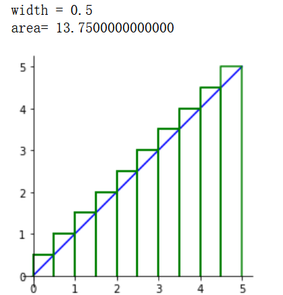
You can see that the bottom edge of each rectangle is b/n, the height is b/n, 2b/n

So area:

The teacher's calculation is to directly give the calculation formula of triangle width * height / 2

So area:

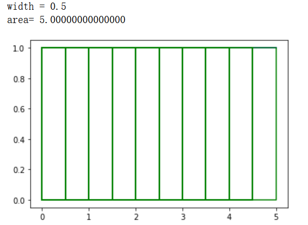
3. F (x) = 1, a = 0, B arbitrary

the measure of area:

x = symbols('x')
expr = x**0

DrawXY(0,5,100,expr,'blue','',plt)
DrawRects(0,5,10,expr,'green',plt)
#plt.legend(loc='lower right')
plt.show()

 

​

 

Here the teacher summarized the mode of definite integral

​

 

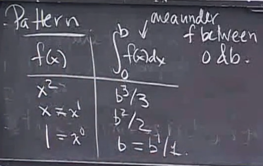
Guess:

Check:

x = symbols('x')
expr = x**3
b = 1
n = 100
DrawXY(0,b,80,expr,'blue','',plt)
DrawRects(0,b,n,expr,'green',plt)
area1 = b / 4
print ('area1 = b**4/4 = ' , area1 )
#plt.legend(loc='lower right')
plt.show()

 

​

 

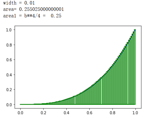
We can see that when n is set to 100, the result is close to the guess value. When n is larger, the result should be closer to 0.25.

x = symbols('x')
expr = x**3
b = 1
n = 300
DrawXY(0,b,80,expr,'blue','',plt)
DrawRects(0,b,n,expr,'green',plt)
area1 = b / 4
print ('area1 = b**4/4 = ' , area1 )
#plt.legend(loc='lower right')
plt.show()

 

​

 

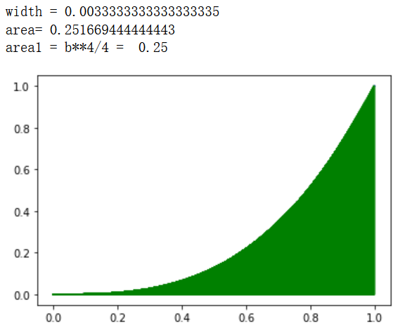
It can be seen that when n takes 300, the result is indeed closer to 0.25

3, Sign of definite integral (Riemannian sum)

1. The usual steps of solving definite integral

 

The sum of all the function values at these intervals is the area (the value of the definite integral)

(the former is Riemann sum, whenWhen it approaches 0, it becomes the latter (Leibniz's limit evaluation)

Integral can be expressed as cumulative sum

Let the time t (yr), and the function f(t) ($/yr) with t expresses the borrowing rate (how much money to borrow every day). Suppose you borrow money every day, so there is

I borrowed money on the 45th day. How much did I borrow? Use this formula to calculate  ($)

If you want to calculate the money borrowed throughout the year, use the following formula

(note that the unit of t is year)

The interest is compounded. How much money do you owe the bank at the end of that year?

The interest rate is R (can be 0.05/yr), P (borrowed principal) after time t, and the money owed is

How much do you owe a year?