chart

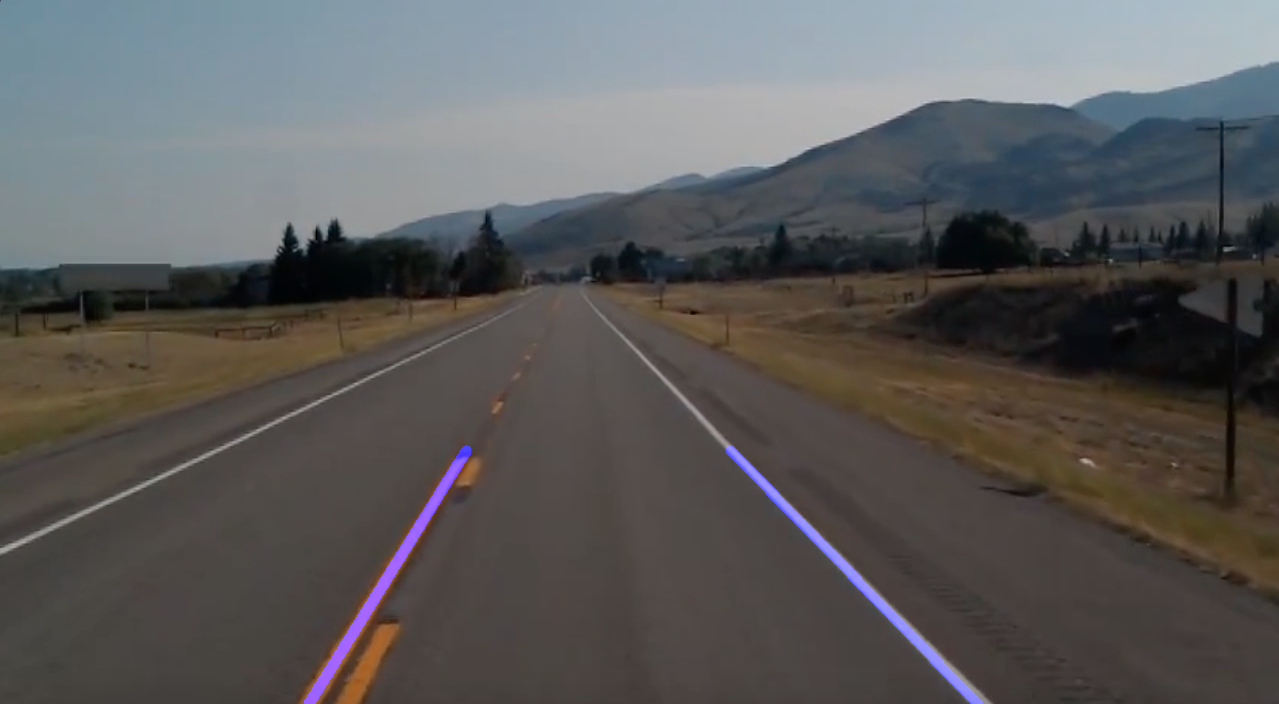
Next to the code section, here we will explain in detail what the HoughLinesP parameter means and how to use it.

lines = cv2.HoughLinesP(cropped_image,2,np.pi/180,100,np.array([]),minLineLength=40,maxLineGap=5)

The first parameter is the picture we want to check
Hough accumulator array
The second and third parameters define how our Hough coordinates divide the bin, or the precision of the lattice.We voted through the bin grid with a curve, and we determined the values of p and theta based on the number of votes.2 means our cell width is in pixels.

chart

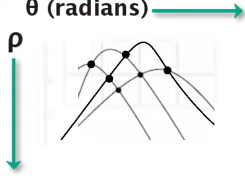
We can divide the cells by the following figure. As long as the curve passes, the cells will be voted. We record the number of votes and record the most as a parameter.

chart

chart

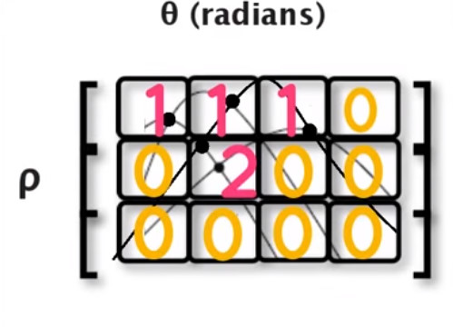
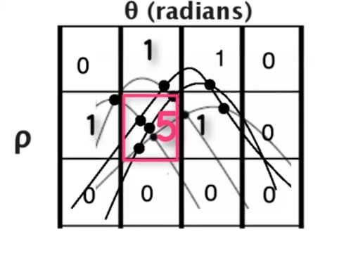
If the definition size is too large, the precision will be lost, and if the definition grid size is too small, the accuracy will increase the calculation time.

The next parameter, 100, indicates that the line we voted for more than 100 is the line we are looking for.That is, more than 100 lines need to intersect in the bin cell to be the parameter we are looking for.

minLineLength gives 40 to indicate that our check line length cannot be less than 40 pixel s
maxLineGap=5 cannot be greater than 5 pixel as a line break

Define method for displaying lane lines

def disply_lines(image,lines):
    pass

Display the found lane lines by defining a function.

line_image = disply_lines(lane_image,lines)

View Detection Lane Line Data Structure

def disply_lines(image,lines):
    line_image = np.zeros_like(image)
    if lines is not None:
        for line in lines:
            print(line)

First, define a matrix of the same size as the original to draw the found Lane lines. Let's first determine if the lane lines have been found. Lines return value should not be a matrix. We can simply print it to see the effect.

[[704 418 927 641]]
[[704 426 791 516]]
[[320 703 445 494]]
[[585 301 663 381]]
[[630 341 670 383]]

Detect lane lines

Looking at the two-dimensional array of data structures [[x1,y1,x2,y2]]], we need to convert it to one-dimensional data [x1,y1,x2,y2]

def disply_lines(image,lines):
    line_image = np.zeros_like(image)
    if lines is not None:
        for line in lines:
            x1,y1,x2,y2 = line.reshape(4)
            cv2.line(line_image,(x1,y1),(x2,y2),(255,0,0),10)
    return line_image

line_image = disply_lines(lane_image,lines)
cv2.imshow('result',line_image)

Detector Line

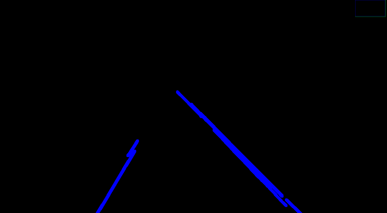
Synthetic effect

combo_image = cv2.addWeighted(lane_image,0.8, line_image, 1, 1,1)

For synthetic pictures, we combine two pictures by overlaying them with a certain weight.

chart

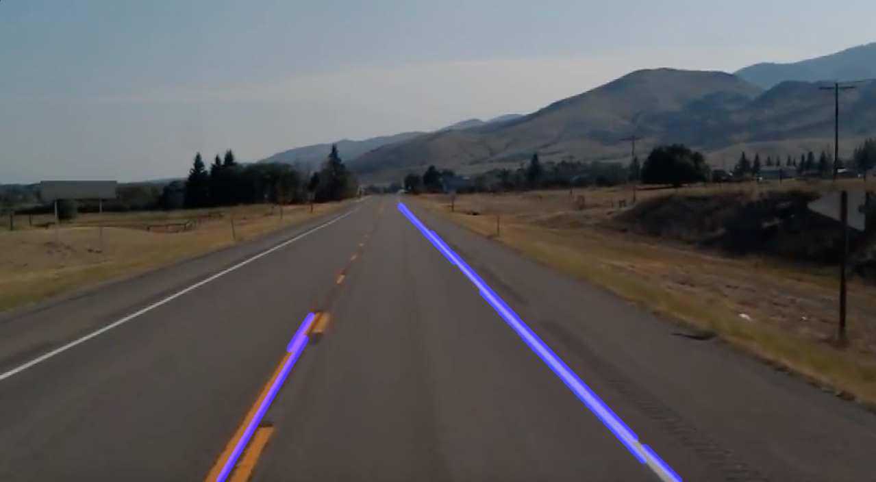
optimization

By learning whether the lane lines detected by the Hough transform are not smooth enough, we need to optimize them. The basic idea is to average the slope and intercept of these lines and then draw all the detected points onto a straight line.

averaged_lines = average_slope_intercept(lane_image,lines);

First, we define our function to receive road pictures and detection points as parameters.

def average_slope_intercept(image,lines):
    left_fit = []
    right_fit = []
    for line in lines:
        x1, y1, x2, y2 = line.reshape(4)
        parameters = np.polyfit((x1,x2),(y1,y2),1)
        print(parameters)

Here, two arrays, left_fit and right_fit, are defined to store the points of the lane lines on both sides of the road. Let's print the slope and intercept of the lines. By entering two points with the polyfit method provided by numpy, we can get the slope and intercept of the line through these points.

[   1. -286.]
[   1.03448276 -302.27586207]
[  -1.672 1238.04 ]
[   1.02564103 -299.

def average_slope_intercept(image,lines):
    left_fit = []
    right_fit = []
    for line in lines:
        x1, y1, x2, y2 = line.reshape(4)
        parameters = np.polyfit((x1,x2),(y1,y2),1)
        # print(parameters)
        slope = parameters[0]
        intercept = parameters[1]
        if slope < 0:
            left_fit.append((slope,intercept))
        else:
            right_fit.append((slope,intercept))
        print(left_fit)
        print(right_fit)

Because the slopes of the left and right lines are different, we can divide the points into right and left linear matrices based on the slopes.

    left_fit_average = np.average(left_fit,axis=0)
    right_fit_average = np.average(right_fit,axis=0)

They then draw to get their average slope and intercept.

[  -1.61019355 1201.00387097]
[   1.0243751  -298.80648538]

def make_coordinates(image, line_parameters):
    slope, intercept = line_parameters
    print(image.shape)
    return 

Let's output the size of the picture. Our picture starts with its upper left corner as the origin 0,0, so we don't need to draw all of it to intercept a part of it, because we draw straight lines up from more than 700 at the bottom of the picture.
! [Fig. https://upload-images.jianshu.io/upload_images/8207483-367e149bfb5a5165.jpg?imageMogr2/auto-orient/strip%7CimageView2/2/w/1240)

chart

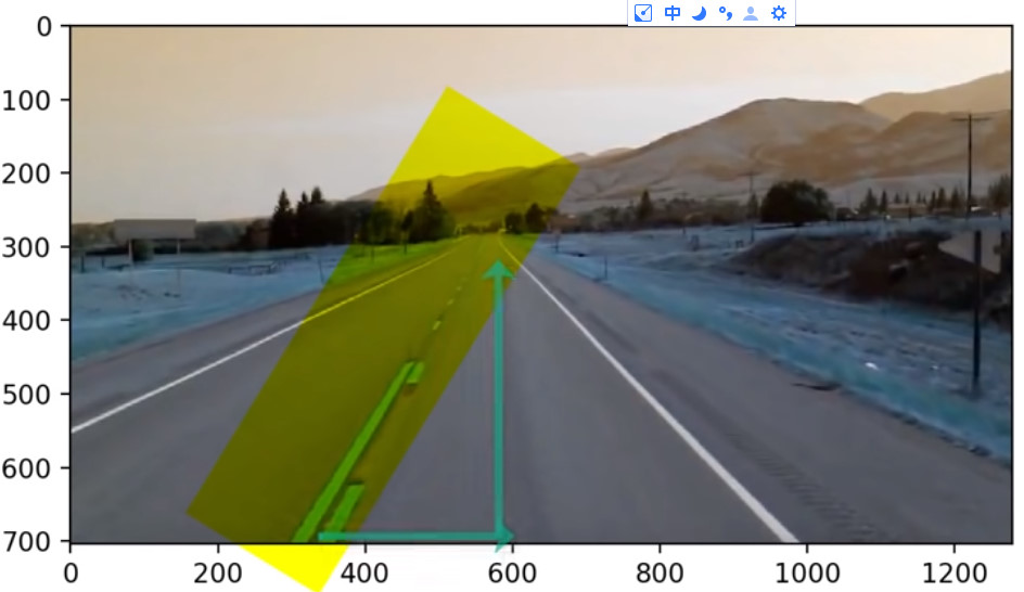
(704, 1279, 3)
(704, 1279, 3)

    left_line = make_coordinates(image, left_fit_average)
    right_line = make_coordinates(image, right_fit_average)

def make_coordinates(image, line_parameters):
    slope, intercept = line_parameters
    y1 = image.shape[0]
    y2 = int(y1*(3/5)) 
    x1 = int((y1 - intercept)/slope)
    x2 = int((y2 - intercept)/slope)
    # print(image.shape)
    return np.array([x1,y1,x2,y2])

So the line starts and ends when we give y1,y2, and then x is calculated from y by the slope and intercept of the equation.

averaged_lines = average_slope_intercept(lane_image,lines);
line_image = disply_lines(lane_image,averaged_lines)
combo_image = cv2.addWeighted(lane_image,0.8, line_image, 1, 1,1)

cv2.imshow('result',combo_image)

result_optimize.png