Untitled-0720 records a complete machine learning project

Posted by Centrek on Sat, 15 Jan 2022 14:46:46 +0100

#Effective switching between py2 and py3
from __future__ import division, print_function, unicode_literals

import numpy as np
import os

preface

When carrying out a complete machine learning project, the following steps need to be completed

Understand the complete project
get data
Discover visual data, discover rules
Find the appropriate machine learning algorithm and prepare the corresponding data
Select the model for training
Fine tuning model
Give solutions
Deployment, monitoring and maintenance

First, understand the data

Model objective: to establish a California house price prediction model based on California census data
Data content: population, median income, median house price and other indicators of each block group
Delimitation problem: building a model is not the ultimate goal, predicting house prices is the goal, and the predicted house prices will be further used in the next investment model
Determine the reference performance P: the error rate calculated manually is about 15%.
Sort out the problem: the type is supervised learning, the multivariable regression problem is carried out, and the goal is prediction
Select performance index: the typical index of regression problem is root mean square error (RMSE)
R M S E = 1 m ∑ i = 1 m ( h ( x ( i ) ) − y ( i ) ) 2 RMSE\,\,=\,\,\sqrt{\frac{1}{m}\sum_{i=1}^m{\left( h\left( x^{\left( i \right)} \right) -y^{\left( i \right)} \right) ^2}} RMSE=m1∑i=1m(h(x(i))−y(i))2
Suppose there are many abnormal blocks. At this point, you may need to use the average absolute error
M A E ( X , h ) = 1 m ∑ i = 1 m ∣ h ( x ( i ) ) − y ( i ) ∣ MAE\left( X,h \right) =\frac{1}{m}\sum_{i=1}^m{|h\left( x^{\left( i \right)} \right) -y^{\left( i \right)}|} MAE(X,h)=m1∑i=1m∣h(x(i))−y(i)∣

np.random.seed(42)

%matplotlib inline

import matplotlib as mpl
import matplotlib.pyplot as plt
mpl.rc("axes",labelsize=14)
mpl.rc('xtick',labelsize=12)
mpl.rc("ytick",labelsize=12)


#Establish storage file location
ROOT ='.'
DATE ='0720'
IMAGE = os.path.join(ROOT,'images',DATE)
os.makedirs(IMAGE,exist_ok  =True)

# Create save map location
def save_fig(fig_id, tight_layout=True, fig_extension="png", resolution=300):
    path = os.path.join(IMAGE, fig_id + "." + fig_extension)
    print("Saving figure", fig_id)
    if tight_layout:
        plt.tight_layout()
    plt.savefig(path, format=fig_extension, dpi=resolution)

GET DATA

import pandas as pd
import os
import tarfile

housing = pd.read_csv('./housing.csv')
housing.head()

	longitude	latitude	housing_median_age	total_rooms	total_bedrooms	population	households	median_income	median_house_value	ocean_proximity
0	-122.23	37.88	41.0	880.0	129.0	322.0	126.0	8.3252	452600.0	NEAR BAY
1	-122.22	37.86	21.0	7099.0	1106.0	2401.0	1138.0	8.3014	358500.0	NEAR BAY
2	-122.24	37.85	52.0	1467.0	190.0	496.0	177.0	7.2574	352100.0	NEAR BAY
3	-122.25	37.85	52.0	1274.0	235.0	558.0	219.0	5.6431	341300.0	NEAR BAY
4	-122.25	37.85	52.0	1627.0	280.0	565.0	259.0	3.8462	342200.0	NEAR BAY

View specific information of data

housing.info()

<class 'pandas.core.frame.DataFrame'>
RangeIndex: 20640 entries, 0 to 20639
Data columns (total 10 columns):
 #   Column              Non-Null Count  Dtype  
---  ------              --------------  -----  
 0   longitude           20640 non-null  float64
 1   latitude            20640 non-null  float64
 2   housing_median_age  20640 non-null  float64
 3   total_rooms         20640 non-null  float64
 4   total_bedrooms      20433 non-null  float64
 5   population          20640 non-null  float64
 6   households          20640 non-null  float64
 7   median_income       20640 non-null  float64
 8   median_house_value  20640 non-null  float64
 9   ocean_proximity     20640 non-null  object 
dtypes: float64(9), object(1)
memory usage: 1.6+ MB

0-1 longitude&latitude
2- median age
3 - number of houses
4 - number of bedrooms
5 - population
6 - number of accounts
7 - median income
8 - median house price
9 - sea view

Combing scalar data

housing['ocean_proximity'].value_counts()

<1H OCEAN     9136
INLAND        6551
NEAR OCEAN    2658
NEAR BAY      2290
ISLAND           5
Name: ocean_proximity, dtype: int64

landlocked
offshore
Near Port
islands

descriptive statistics

housing.describe()

	longitude	latitude	housing_median_age	total_rooms	total_bedrooms	population	households	median_income	median_house_value
count	20640.000000	20640.000000	20640.000000	20640.000000	20433.000000	20640.000000	20640.000000	20640.000000	20640.000000
mean	-119.569704	35.631861	28.639486	2635.763081	537.870553	1425.476744	499.539680	3.870671	206855.816909
std	2.003532	2.135952	12.585558	2181.615252	421.385070	1132.462122	382.329753	1.899822	115395.615874
min	-124.350000	32.540000	1.000000	2.000000	1.000000	3.000000	1.000000	0.499900	14999.000000
25%	-121.800000	33.930000	18.000000	1447.750000	296.000000	787.000000	280.000000	2.563400	119600.000000
50%	-118.490000	34.260000	29.000000	2127.000000	435.000000	1166.000000	409.000000	3.534800	179700.000000
75%	-118.010000	37.710000	37.000000	3148.000000	647.000000	1725.000000	605.000000	4.743250	264725.000000
max	-114.310000	41.950000	52.000000	39320.000000	6445.000000	35682.000000	6082.000000	15.000100	500001.000000

%matplotlib inline
import matplotlib.pyplot as plt
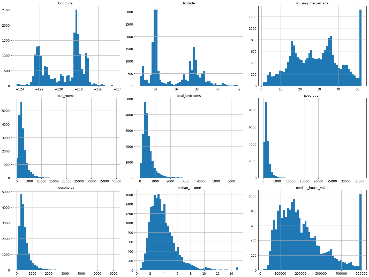
housing.hist(bins=50, figsize=(20,15))
save_fig("attribute_histogram_plots")
plt.show()

Saving figure attribute_histogram_plots

np.random.seed(42)

Training data: Division

from sklearn.model_selection import train_test_split
train_set, test_set = train_test_split(housing, test_size=0.2, random_state=42)
#test_size=0.2 test set accounts for 20%

####################! [Please add picture description]( https://csdn-img-blog.oss-cn-beijing.aliyuncs.com/cb73e934f4cb449291811189491fcb57.png?x-oss-process=image/watermark,type_ZmFuZ3poZW5naGVpdGk,shadow_10,text_aHR0cHM6Ly9ibG9nLmNzZG4ubmV0L3dlaXhpbl80NTUzNjkzNg==,size_16,color_FFFFFF,t_70)
#############################################################################
# train_set, test_set = train_test_split(housing, test_size=0.2, random_state=42)

#################################################################################################
train_set.head(5)

	longitude	latitude	housing_median_age	total_rooms	total_bedrooms	population	households	median_income	median_house_value	ocean_proximity
14196	-117.03	32.71	33.0	3126.0	627.0	2300.0	623.0	3.2596	103000.0	NEAR OCEAN
8267	-118.16	33.77	49.0	3382.0	787.0	1314.0	756.0	3.8125	382100.0	NEAR OCEAN
17445	-120.48	34.66	4.0	1897.0	331.0	915.0	336.0	4.1563	172600.0	NEAR OCEAN
14265	-117.11	32.69	36.0	1421.0	367.0	1418.0	355.0	1.9425	93400.0	NEAR OCEAN
2271	-119.80	36.78	43.0	2382.0	431.0	874.0	380.0	3.5542	96500.0	INLAND

test_set.head()

	longitude	latitude	housing_median_age	total_rooms	total_bedrooms	population	households	median_income	median_house_value	ocean_proximity
20046	-119.01	36.06	25.0	1505.0	NaN	1392.0	359.0	1.6812	47700.0	INLAND
3024	-119.46	35.14	30.0	2943.0	NaN	1565.0	584.0	2.5313	45800.0	INLAND
15663	-122.44	37.80	52.0	3830.0	NaN	1310.0	963.0	3.4801	500001.0	NEAR BAY
20484	-118.72	34.28	17.0	3051.0	NaN	1705.0	495.0	5.7376	218600.0	<1H OCEAN
9814	-121.93	36.62	34.0	2351.0	NaN	1063.0	428.0	3.7250	278000.0	NEAR OCEAN

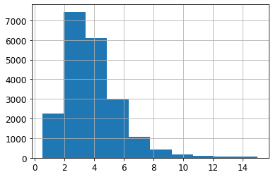
housing["median_income"].hist()

<AxesSubplot:>

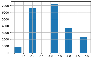
housing['income_cat']= pd.cut(housing['median_income'],bins=[0., 1.5, 3.0, 4.5, 6., np.inf],labels=[1, 2, 3, 4, 5])

housing['income_cat'].value_counts()

3    7236
2    6581
4    3639
5    2362
1     822
Name: income_cat, dtype: int64

housing['income_cat'].hist()

<AxesSubplot:>

https://blog.csdn.net/Cicome/article/details/79153268

Stratified sampling using structured shufflesplit

from sklearn.model_selection import StratifiedShuffleSplit

split = StratifiedShuffleSplit(n_splits=1, test_size=0.2, random_state=42)
for train_index, test_index in split.split(housing, housing["income_cat"]):
    strat_train_set = housing.loc[train_index]
    strat_test_set = housing.loc[test_index]

###########################################################################
train_index, test_index in split.split(housing, housing["income_cat"])
print(len(train_index),len(test_index))

16512 4128


D:\anaconda\lib\site-packages\ipykernel_launcher.py:2: VisibleDeprecationWarning: Creating an ndarray from ragged nested sequences (which is a list-or-tuple of lists-or-tuples-or ndarrays with different lengths or shapes) is deprecated. If you meant to do this, you must specify 'dtype=object' when creating the ndarray
  
D:\anaconda\lib\site-packages\ipykernel_launcher.py:2: DeprecationWarning: elementwise comparison failed; this will raise an error in the future.

strat_test_set["income_cat"].value_counts() / len(strat_test_set)

3    0.350533
2    0.318798
4    0.176357
5    0.114583
1    0.039729
Name: income_cat, dtype: float64

for set_ in (strat_train_set, strat_test_set):
    set_.drop("income_cat", axis=1, inplace=True)

Data exploration

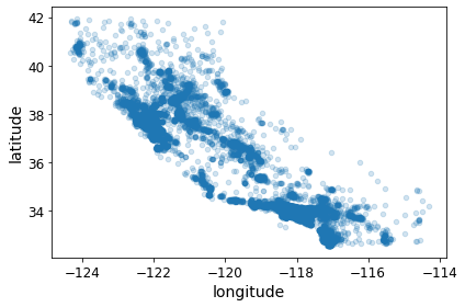
housing = strat_train_set.copy()

housing.plot(kind="scatter", x="longitude", y="latitude",alpha=0.2)
save_fig("bad_visualization_plot")

Saving figure bad_visualization_plot

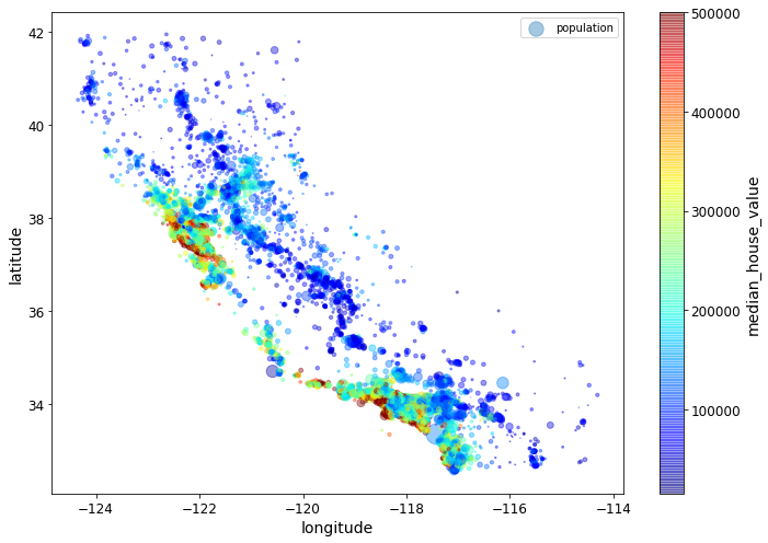
housing.plot(kind="scatter", x="longitude", y="latitude", alpha=0.4,
    s=housing["population"]/100, label="population", figsize=(10,7),
    c="median_house_value", cmap=plt.get_cmap("jet"), colorbar=True,
    sharex=False)
plt.legend()
save_fig("housing_prices_scatterplot")

Saving figure housing_prices_scatterplot

import os
import tarfile
import urllib.request

PROJECT_ROOT_DIR = "."

images_path = os.path.join(PROJECT_ROOT_DIR, "images", "end_to_end_project")
os.makedirs(images_path, exist_ok=True)
DOWNLOAD_ROOT = "https://raw.githubusercontent.com/ageron/handson-ml/master/"
filename = "california.png"
print("Downloading", filename)
url = DOWNLOAD_ROOT + "images/end_to_end_project/" + filename
urllib.request.urlretrieve(url, os.path.join(images_path, filename))

Downloading california.png





('.\\images\\end_to_end_project\\california.png',
 <http.client.HTTPMessage at 0x22a301f6648>)

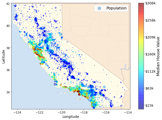
import matplotlib.image as mpimg

california_img=mpimg.imread(PROJECT_ROOT_DIR + '/images/end_to_end_project/california.png')
ax = housing.plot(kind="scatter", x="longitude", y="latitude", figsize=(10,7),
                       s=housing['population']/100, label="Population",
                       c="median_house_value", cmap=plt.get_cmap("jet"),
                       colorbar=False, alpha=0.4,
                      )
plt.imshow(california_img, extent=[-124.55, -113.80, 32.45, 42.05], alpha=0.5,
           cmap=plt.get_cmap("jet"))
plt.ylabel("Latitude", fontsize=14)
plt.xlabel("Longitude", fontsize=14)


prices = housing["median_house_value"]
tick_values = np.linspace(prices.min(), prices.max(), 11)
cbar = plt.colorbar()
cbar.ax.set_yticklabels(["$%dk"%(round(v/1000)) for v in tick_values], fontsize=14)
cbar.set_label('Median House Value', fontsize=16)

plt.legend(fontsize=16)
save_fig("california_housing_prices_plot")
plt.show()

D:\anaconda\lib\site-packages\ipykernel_launcher.py:18: UserWarning: FixedFormatter should only be used together with FixedLocator


Saving figure california_housing_prices_plot

correlation coefficient

corr_matrix = housing.corr()

#Correlation between each attribute and median house price
corr_matrix["median_house_value"].sort_values(ascending=False)

median_house_value    1.000000
median_income         0.688075
total_rooms           0.134153
housing_median_age    0.105623
households            0.065843
total_bedrooms        0.049686
population           -0.024650
longitude            -0.045967
latitude             -0.144160
Name: median_house_value, dtype: float64

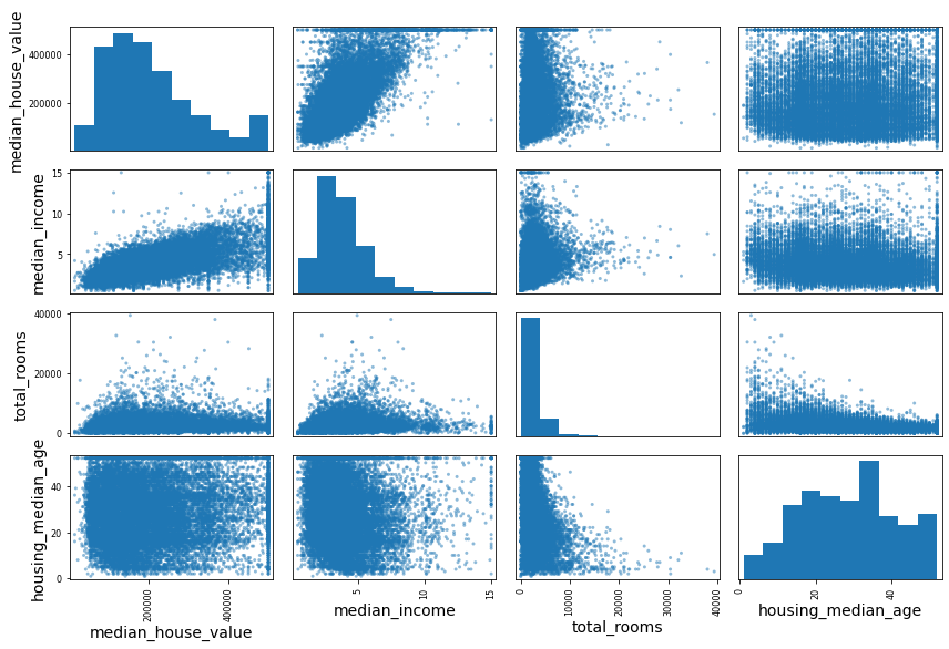
from pandas.plotting import scatter_matrix


attributes = ["median_house_value", "median_income", "total_rooms",
              "housing_median_age"]
scatter_matrix(housing[attributes], figsize=(12, 8))
save_fig("scatter_matrix_plot")

Saving figure scatter_matrix_plot

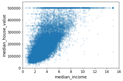
housing.plot(kind="scatter", x="median_income", y="median_house_value",
             alpha=0.1)
plt.axis([0, 16, 0, 550000])
save_fig("income_vs_house_value_scatterplot")

Saving figure income_vs_house_value_scatterplot

Attribute combination test

housing["rooms_per_household"] = housing["total_rooms"]/housing["households"]
housing["bedrooms_per_room"] = housing["total_bedrooms"]/housing["total_rooms"]
housing["population_per_household"]=housing["population"]/housing["households"]

corr_matrix = housing.corr()
corr_matrix["median_house_value"].sort_values(ascending=False)

median_house_value          1.000000
median_income               0.688075
rooms_per_household         0.151948
total_rooms                 0.134153
housing_median_age          0.105623
households                  0.065843
total_bedrooms              0.049686
population_per_household   -0.023737
population                 -0.024650
longitude                  -0.045967
latitude                   -0.144160
bedrooms_per_room          -0.255880
Name: median_house_value, dtype: float64

median_house_value

median_income 0.687160
bedrooms_per_room -0.259984
rooms_per_household 0.146285
total_rooms 0.135097
housing_median_age 0.114110

Prepare the data for Machine Learning algorithms

It is convenient to convert duplicate data on any data set (for example, the next time you get a new data set).
Slowly build a conversion function library, which can be reused in future projects.

housing = strat_train_set.drop("median_house_value", axis=1) # It does not affect the original data, but only establishes a backup
housing_labels = strat_train_set["median_house_value"].copy()

Data cleaning

For missing values:

Remove the corresponding block;
Remove the entire attribute;
Assign values (0, mean, median, etc.).

housing.dropna(subset=["total_bedrooms"]) # Option 1
housing.drop("total_bedrooms", axis=1) # Option 2
median = housing["total_bedrooms"].median()
housing["total_bedrooms"].fillna(median) # Option 3

If you select option 3, you need to calculate the median of the training set, fill in the missing values of the training set with the median, and don't forget to save
The median. When the test set is used to evaluate the system later, the missing value in the test set needs to be replaced, and it can also be used to replace the new value in real time
Missing value in data

Scikit learn provides a convenient class to handle missing values: Imputer

from sklearn.preprocessing import Imputer
imputer = Imputer(strategy="median")
housing_num = housing.drop("ocean_proximity", axis=1)
imputer.fit(housing_num)
imputer.statistics_
X = imputer.transform(housing_num)
housing_tr = pd.DataFrame(X, columns=housing_num.columns)

sample_incomplete_rows = housing[housing.isnull().any(axis=1)].head()
#df.isnull().any() determines which columns contain missing values
sample_incomplete_rows

	longitude	latitude	housing_median_age	total_rooms	total_bedrooms	population	households	median_income	ocean_proximity
4629	-118.30	34.07	18.0	3759.0	NaN	3296.0	1462.0	2.2708	<1H OCEAN
6068	-117.86	34.01	16.0	4632.0	NaN	3038.0	727.0	5.1762	<1H OCEAN
17923	-121.97	37.35	30.0	1955.0	NaN	999.0	386.0	4.6328	<1H OCEAN
13656	-117.30	34.05	6.0	2155.0	NaN	1039.0	391.0	1.6675	INLAND
19252	-122.79	38.48	7.0	6837.0	NaN	3468.0	1405.0	3.1662	<1H OCEAN

Visible total_ Missing value for bedrooms

So use the median instead

Just take the median of all the features in the data set together

Saved in impater

Here we use exceptions to deal with the problem of sklearn version change

try:
    from sklearn.impute import SimpleImputer # Scikit-Learn 0.20+
except ImportError:
    from sklearn.preprocessing import Imputer as SimpleImputer
    
imputer = SimpleImputer(strategy="median")

housing_num = housing.drop('ocean_proximity', axis=1)#Delete the scalar data, otherwise you can't calculate the median uniformly

imputer.fit(housing_num)

SimpleImputer(strategy='median')

#Look at the data
imputer.statistics_

array([-118.51  ,   34.26  ,   29.    , 2119.5   ,  433.    , 1164.    ,
        408.    ,    3.5409])

X = imputer.transform(housing_num)#Replace missing values with median
housing_num

	longitude	latitude	housing_median_age	total_rooms	total_bedrooms	population	households	median_income
17606	-121.89	37.29	38.0	1568.0	351.0	710.0	339.0	2.7042
18632	-121.93	37.05	14.0	679.0	108.0	306.0	113.0	6.4214
14650	-117.20	32.77	31.0	1952.0	471.0	936.0	462.0	2.8621
3230	-119.61	36.31	25.0	1847.0	371.0	1460.0	353.0	1.8839
3555	-118.59	34.23	17.0	6592.0	1525.0	4459.0	1463.0	3.0347
...	...	...	...	...	...	...	...	...
6563	-118.13	34.20	46.0	1271.0	236.0	573.0	210.0	4.9312
12053	-117.56	33.88	40.0	1196.0	294.0	1052.0	258.0	2.0682
13908	-116.40	34.09	9.0	4855.0	872.0	2098.0	765.0	3.2723
11159	-118.01	33.82	31.0	1960.0	380.0	1356.0	356.0	4.0625
15775	-122.45	37.77	52.0	3095.0	682.0	1269.0	639.0	3.5750

16512 rows × 8 columns

housing_tr = pd.DataFrame(X, columns=housing_num.columns,
                          index=housing.index)

Scalar data processing

housing_cat = housing[['ocean_proximity']]
housing_cat.head(10)

	ocean_proximity
17606	<1H OCEAN
18632	<1H OCEAN
14650	NEAR OCEAN
3230	INLAND
3555	<1H OCEAN
19480	INLAND
8879	<1H OCEAN
13685	INLAND
4937	<1H OCEAN
4861	<1H OCEAN

try:
    from sklearn.preprocessing import OrdinalEncoder # just to raise an ImportError if Scikit-Learn < 0.20
    from sklearn.preprocessing import OneHotEncoder
except ImportError:
    from future_encoders import OneHotEncoder 

cat_encoder = OneHotEncoder(sparse=False)
housing_cat_1hot = cat_encoder.fit_transform(housing_cat)
housing_cat_1hot

array([[1., 0., 0., 0., 0.],
       [1., 0., 0., 0., 0.],
       [0., 0., 0., 0., 1.],
       ...,
       [0., 1., 0., 0., 0.],
       [1., 0., 0., 0., 0.],
       [0., 0., 0., 1., 0.]])

housing.columns

Index(['longitude', 'latitude', 'housing_median_age', 'total_rooms',
       'total_bedrooms', 'population', 'households', 'median_income',
       'ocean_proximity'],
      dtype='object')

Create your own class

Custom converter:

Create a class that implements fit()[return self], transform(), and fit_transform()

By adding TransformerMixin as the base class (parent class), you can easily get fit_transform().

In addition, if you add BaseEstimator as the base class (parent class) (and avoid using * args and * * kargs in the constructor), you can get two additional methods (get_params() and set)_ params() )，

Both of them can be easily adjusted automatically

The sklearn project can be regarded as a big tree. Various estimators are fruits, and the backbone supporting these estimators is one of the few base classes. Several common classes are BaseEstimator, BaseSGD, ClassifierMixin, RegressorMixin, and so on. [origin]https://www.cnblogs.com/learn-the-hard-way/p/12532888.html

np.c_ Connect several array s together

from sklearn.base import BaseEstimator, TransformerMixin

# get the right column indices: safer than hard-coding indices 3, 4, 5, 6
rooms_ix, bedrooms_ix, population_ix, household_ix = [
    list(housing.columns).index(col)
    for col in ("total_rooms", "total_bedrooms", "population", "households")]

class CombinedAttributesAdder(BaseEstimator, TransformerMixin):
    def __init__(self, add_bedrooms_per_room = True): # no *args or **kwargs
        self.add_bedrooms_per_room = add_bedrooms_per_room
    def fit(self, X, y=None):
        return self  # nothing else to do
    def transform(self, X, y=None):
        rooms_per_household = X[:, rooms_ix] / X[:, household_ix]
        population_per_household = X[:, population_ix] / X[:, household_ix]
        if self.add_bedrooms_per_room:
            bedrooms_per_room = X[:, bedrooms_ix] / X[:, rooms_ix]
            return np.c_[X, rooms_per_household, population_per_household,
                         bedrooms_per_room]
        #  np.c_  Connect several array s together
        else:
            return np.c_[X, rooms_per_household, population_per_household]

attr_adder = CombinedAttributesAdder(add_bedrooms_per_room=False)
housing_extra_attribs = attr_adder.transform(housing.values)

Another method: FunctionTransformer

from sklearn.preprocessing import FunctionTransformer

def add_extra_features(X, add_bedrooms_per_room=True):
    rooms_per_household = X[:, rooms_ix] / X[:, household_ix]
    population_per_household = X[:, population_ix] / X[:, household_ix]
    if add_bedrooms_per_room:
        bedrooms_per_room = X[:, bedrooms_ix] / X[:, rooms_ix]
        return np.c_[X, rooms_per_household, population_per_household,
                     bedrooms_per_room]
    else:
        return np.c_[X, rooms_per_household, population_per_household]

attr_adder = FunctionTransformer(add_extra_features, validate=False,
                                 kw_args={"add_bedrooms_per_room": False})
housing_extra_attribs = attr_adder.fit_transform(housing.values)

housing_extra_attribs = pd.DataFrame(
    housing_extra_attribs,
    columns=list(housing.columns)+["rooms_per_household", "population_per_household"],
    index=housing.index)
housing_extra_attribs.columns

Index(['longitude', 'latitude', 'housing_median_age', 'total_rooms',
       'total_bedrooms', 'population', 'households', 'median_income',
       'ocean_proximity', 'rooms_per_household', 'population_per_household'],
      dtype='object')

from sklearn.pipeline import Pipeline
from sklearn.preprocessing import StandardScaler

num_pipeline = Pipeline([
        ('imputer', SimpleImputer(strategy="median")),#1.Remove missing values  #Execute imputer = simpleimputer (strategy = "intermediate") imputer fit(housing_num)
        ('attribs_adder', FunctionTransformer(add_extra_features, validate=False)),#2.Add attribute     #FunctionTransformer(add_extra_features, validate=False)
        ('std_scaler', StandardScaler()),#3. Feature scaling
    ])

housing_num_tr = num_pipeline.fit_transform(housing_num)

Index(['longitude', 'latitude', 'housing_median_age', 'total_rooms',
       'total_bedrooms', 'population', 'households', 'median_income'],
      dtype='object')

Feature scaling

An important link in machine learning
Do not update temporarily

Conversion pipeline

Use pipline to execute programs in a certain order

try:
    from sklearn.compose import ColumnTransformer
except ImportError:
    from future_encoders import ColumnTransformer # Scikit-Learn < 0.20

num_attribs = list(housing_num)
cat_attribs = ["ocean_proximity"]

full_pipeline = ColumnTransformer([
        ("num", num_pipeline, num_attribs),
        ("cat", OneHotEncoder(), cat_attribs),
    ])

housing_prepared = full_pipeline.fit_transform(housing)

housing_prepared

array([[-1.15604281,  0.77194962,  0.74333089, ...,  0.        ,
         0.        ,  0.        ],
       [-1.17602483,  0.6596948 , -1.1653172 , ...,  0.        ,
         0.        ,  0.        ],
       [ 1.18684903, -1.34218285,  0.18664186, ...,  0.        ,
         0.        ,  1.        ],
       ...,
       [ 1.58648943, -0.72478134, -1.56295222, ...,  0.        ,
         0.        ,  0.        ],
       [ 0.78221312, -0.85106801,  0.18664186, ...,  0.        ,
         0.        ,  0.        ],
       [-1.43579109,  0.99645926,  1.85670895, ...,  0.        ,
         1.        ,  0.        ]])

housing_prepared.shape

(16512, 16)

from sklearn.base import BaseEstimator, TransformerMixin

# Create a class to select numerical or categorical columns 
class OldDataFrameSelector(BaseEstimator, TransformerMixin):
    def __init__(self, attribute_names):
        self.attribute_names = attribute_names
    def fit(self, X, y=None):
        return self
    def transform(self, X):
        return X[self.attribute_names].values

num_attribs = list(housing_num)
cat_attribs = ["ocean_proximity"]

old_num_pipeline = Pipeline([
        ('selector', OldDataFrameSelector(num_attribs)),
        ('imputer', SimpleImputer(strategy="median")),
        ('attribs_adder', FunctionTransformer(add_extra_features, validate=False)),
        ('std_scaler', StandardScaler()),
    ])

old_cat_pipeline = Pipeline([
        ('selector', OldDataFrameSelector(cat_attribs)),
        ('cat_encoder', OneHotEncoder(sparse=False)),
    ])

from sklearn.pipeline import FeatureUnion

old_full_pipeline = FeatureUnion(transformer_list=[
        ("num_pipeline", old_num_pipeline),
        ("cat_pipeline", old_cat_pipeline),
    ])

old_housing_prepared = old_full_pipeline.fit_transform(housing)
old_housing_prepared

array([[-1.15604281,  0.77194962,  0.74333089, ...,  0.        ,
         0.        ,  0.        ],
       [-1.17602483,  0.6596948 , -1.1653172 , ...,  0.        ,
         0.        ,  0.        ],
       [ 1.18684903, -1.34218285,  0.18664186, ...,  0.        ,
         0.        ,  1.        ],
       ...,
       [ 1.58648943, -0.72478134, -1.56295222, ...,  0.        ,
         0.        ,  0.        ],
       [ 0.78221312, -0.85106801,  0.18664186, ...,  0.        ,
         0.        ,  0.        ],
       [-1.43579109,  0.99645926,  1.85670895, ...,  0.        ,
         1.        ,  0.        ]])

np.allclose(housing_prepared, old_housing_prepared)

True

Select and train models

from sklearn.linear_model import LinearRegression

lin_reg = LinearRegression()
lin_reg.fit(housing_prepared, housing_labels)

LinearRegression()

some_data=housing.iloc[:5]
some_labels=housing_labels.iloc[:5]
some_data_prepared = full_pipeline.transform(some_data)

print("Predictions:", lin_reg.predict(some_data_prepared))

Predictions: [210644.60459286 317768.80697211 210956.43331178  59218.98886849
 189747.55849879]

from sklearn.metrics import mean_squared_error

housing_predictions = lin_reg.predict(housing_prepared)
lin_mse = mean_squared_error(housing_labels, housing_predictions)
lin_rmse = np.sqrt(lin_mse)
lin_rmse

68628.19819848923

68628.19819848923
The median housing value is between 120000 and 265000
So 68628 is still too big!!!!
It means that there is a problem of under fitting in this model

The main method to repair under fitting is to select a more powerful model, provide better features for the training algorithm, or remove the restrictions on the model. This model has not been regularized, so the last option is excluded. You can try to add more features (for example, logarithm of population), but first let's try a more complex model to see the effect.

Try the decision tree

from sklearn.tree import DecisionTreeRegressor

tree_reg = DecisionTreeRegressor(random_state=42)
tree_reg.fit(housing_prepared, housing_labels)

DecisionTreeRegressor(random_state=42)

housing_predictions = tree_reg.predict(housing_prepared)
tree_mse = mean_squared_error(housing_labels, housing_predictions)
tree_rmse = np.sqrt(tree_mse)
tree_rmse

0.0

RMSE is 0!!!!!!!!!!!!!!!!!!!

Serious over fitting warning!!!!!!!!!!!!!

Before we select the model, we can't touch the test set at all!!!!!!!

Cross validation

from sklearn.model_selection import cross_val_score

scores = cross_val_score(tree_reg, housing_prepared, housing_labels,
                         scoring="neg_mean_squared_error", cv=10)
tree_rmse_scores = np.sqrt(-scores)

Special comments!!!!!!!!!!!!!!
The function used for the cross validation score is the utility function, not the cost function, so the larger the score, the better (negative number)
Calculate - scores before calculating the square root.

def display_scores(scores):
    print("Scores:", scores)
    print("Mean:", scores.mean())
    print("Standard deviation:", scores.std())

display_scores(tree_rmse_scores)

Scores: [70194.33680785 66855.16363941 72432.58244769 70758.73896782
 71115.88230639 75585.14172901 70262.86139133 70273.6325285
 75366.87952553 71231.65726027]
Mean: 71407.68766037929
Standard deviation: 2439.4345041191004

It looks worse than the linear regression model! Note that cross validation not only gives you an assessment of the performance of the model, but also measures the accuracy of the assessment (i.e., its standard deviation).

The score of the decision tree is about 71407, which usually fluctuates by ± 2439.

lin_scores = cross_val_score(lin_reg, housing_prepared, housing_labels,
                         scoring="neg_mean_squared_error", cv=10)
lin_rmse_scores = np.sqrt(-lin_scores)
display_scores(lin_rmse_scores)

Scores: [66782.73843989 66960.118071   70347.95244419 74739.57052552
 68031.13388938 71193.84183426 64969.63056405 68281.61137997
 71552.91566558 67665.10082067]
Mean: 69052.46136345083
Standard deviation: 2731.674001798349

The score of linear regression is about 69052, which usually fluctuates by ± 2731.

The over fitting of decision tree model is very serious, and its performance is worse than that of linear regression model.

from sklearn.ensemble import RandomForestRegressor

forest_reg = RandomForestRegressor(n_estimators=10, random_state=42)
forest_reg.fit(housing_prepared, housing_labels)

RandomForestRegressor(n_estimators=10, random_state=42)

housing_predictions = forest_reg.predict(housing_prepared)
forest_mse = mean_squared_error(housing_labels, housing_predictions)
forest_rmse = np.sqrt(forest_mse)
forest_rmse

21933.31414779769

from sklearn.model_selection import cross_val_score

forest_scores = cross_val_score(forest_reg, housing_prepared, housing_labels,
                                scoring="neg_mean_squared_error", cv=10)
forest_rmse_scores = np.sqrt(-forest_scores)
display_scores(forest_rmse_scores)

Scores: [51646.44545909 48940.60114882 53050.86323649 54408.98730149
 50922.14870785 56482.50703987 51864.52025526 49760.85037653
 55434.21627933 53326.10093303]
Mean: 52583.72407377466
Standard deviation: 2298.353351147122

The score of random forest is about 52583, which usually fluctuates by ± 2298.

The score here refers to the score of the verification set

The score of the training set is lower than that of the verification set, indicating that it is over fitted

Over fitting can be solved by simplifying the model, limiting the model (i.e., regularization), or using more training data.

Before going deep into the random forest, you should try other types of models of machine learning algorithms (support vector machines with different cores, neural networks, etc.),

Don't spend too much time adjusting the super parameters. The goal is to make a list of possible models (two to five).

Replacing models takes precedence over tuning parameters

You should save each tested model so that it can be reused later. To ensure that there are super parameters and training parameters,
And cross validation scores, and actual predicted values. This allows you to compare the scores of different types of models and compare them
More error types. You can use the Python module pickle to easily save the scikit learn model, or use sklearn externals. Joblib, which is more efficient in serializing large NumPy arrays:

from sklearn.externals import joblib
joblib.dump(my_model, "my_model.pkl")
# then
my_model_loaded = joblib.load("my_model.pkl")

Model tuning

Suppose you now have a list of several promising models. You now need to fine tune them. Let's look at several ways to fine tune.

Grid search

One method of fine tuning is to manually adjust the super parameters until a good combination of super parameters is found. It would be very redundant to do so
For a long time, you may not have time to explore multiple combinations.

You should use scikit learn's GridSearchCV to do this search. All you need to do is tell GridSearchCV what super parameters to test and what values to test. GridSearchCV can use cross validation to test all possible combinations of super parameter values. For example, the following code searches for the best combination of RandomForestRegressor hyperparameter values:

from sklearn.model_selection import GridSearchCV

param_grid = [
    # try 12 (3×4) combinations of hyperparameters
    {'n_estimators': [3, 10, 30], 'max_features': [2, 4, 6, 8]},
    # then try 6 (2×3) combinations with bootstrap set as False
    {'bootstrap': [False], 'n_estimators': [3, 10], 'max_features': [2, 3, 4]},
  ]

forest_reg = RandomForestRegressor(random_state=42)
# train across 5 folds, that's a total of (12+6)*5=90 rounds of training 
grid_search = GridSearchCV(forest_reg, param_grid, cv=5,
                           scoring='neg_mean_squared_error', return_train_score=True)
grid_search.fit(housing_prepared, housing_labels)

GridSearchCV(cv=5, estimator=RandomForestRegressor(random_state=42),
             param_grid=[{'max_features': [2, 4, 6, 8],
                          'n_estimators': [3, 10, 30]},
                         {'bootstrap': [False], 'max_features': [2, 3, 4],
                          'n_estimators': [3, 10]}],
             return_train_score=True, scoring='neg_mean_squared_error')

grid_search.best_params_

{'max_features': 8, 'n_estimators': 30}

grid_search.best_estimator_

RandomForestRegressor(max_features=8, n_estimators=30, random_state=42)

cvres = grid_search.cv_results_
for mean_score, params in zip(cvres["mean_test_score"], cvres["params"]):
    print(np.sqrt(-mean_score), params)

63669.11631261028 {'max_features': 2, 'n_estimators': 3}
55627.099719926795 {'max_features': 2, 'n_estimators': 10}
53384.57275149205 {'max_features': 2, 'n_estimators': 30}
60965.950449450494 {'max_features': 4, 'n_estimators': 3}
52741.04704299915 {'max_features': 4, 'n_estimators': 10}
50377.40461678399 {'max_features': 4, 'n_estimators': 30}
58663.93866579625 {'max_features': 6, 'n_estimators': 3}
52006.19873526564 {'max_features': 6, 'n_estimators': 10}
50146.51167415009 {'max_features': 6, 'n_estimators': 30}
57869.25276169646 {'max_features': 8, 'n_estimators': 3}
51711.127883959234 {'max_features': 8, 'n_estimators': 10}
49682.273345071546 {'max_features': 8, 'n_estimators': 30}
62895.06951262424 {'bootstrap': False, 'max_features': 2, 'n_estimators': 3}
54658.176157539405 {'bootstrap': False, 'max_features': 2, 'n_estimators': 10}
59470.40652318466 {'bootstrap': False, 'max_features': 3, 'n_estimators': 3}
52724.9822587892 {'bootstrap': False, 'max_features': 3, 'n_estimators': 10}
57490.5691951261 {'bootstrap': False, 'max_features': 4, 'n_estimators': 3}
51009.495668875716 {'bootstrap': False, 'max_features': 4, 'n_estimators': 10}

pd.DataFrame(grid_search.cv_results_)

	mean_fit_time	std_fit_time	mean_score_time	std_score_time	param_max_features	param_n_estimators	param_bootstrap	params	split0_test_score	split1_test_score	...	mean_test_score	std_test_score	rank_test_score	split0_train_score	split1_train_score	split2_train_score	split3_train_score	split4_train_score	mean_train_score	std_train_score
0	0.066756	0.003714	0.003599	0.000495	2	3	NaN	{'max_features': 2, 'n_estimators': 3}	-3.837622e+09	-4.147108e+09	...	-4.053756e+09	1.519591e+08	18	-1.064113e+09	-1.105142e+09	-1.116550e+09	-1.112342e+09	-1.129650e+09	-1.105559e+09	2.220402e+07
1	0.214235	0.007558	0.010251	0.001075	2	10	NaN	{'max_features': 2, 'n_estimators': 10}	-3.047771e+09	-3.254861e+09	...	-3.094374e+09	1.327062e+08	11	-5.927175e+08	-5.870952e+08	-5.776964e+08	-5.716332e+08	-5.802501e+08	-5.818785e+08	7.345821e+06
2	0.670176	0.023281	0.027710	0.001455	2	30	NaN	{'max_features': 2, 'n_estimators': 30}	-2.689185e+09	-3.021086e+09	...	-2.849913e+09	1.626875e+08	9	-4.381089e+08	-4.391272e+08	-4.371702e+08	-4.376955e+08	-4.452654e+08	-4.394734e+08	2.966320e+06
3	0.117089	0.017003	0.003790	0.000399	4	3	NaN	{'max_features': 4, 'n_estimators': 3}	-3.730181e+09	-3.786886e+09	...	-3.716847e+09	1.631510e+08	16	-9.865163e+08	-1.012565e+09	-9.169425e+08	-1.037400e+09	-9.707739e+08	-9.848396e+08	4.084607e+07
4	0.366152	0.056251	0.009570	0.000797	4	10	NaN	{'max_features': 4, 'n_estimators': 10}	-2.666283e+09	-2.784511e+09	...	-2.781618e+09	1.268607e+08	8	-5.097115e+08	-5.162820e+08	-4.962893e+08	-5.436192e+08	-5.160297e+08	-5.163863e+08	1.542862e+07
5	0.997333	0.014813	0.027328	0.000798	4	30	NaN	{'max_features': 4, 'n_estimators': 30}	-2.387153e+09	-2.588448e+09	...	-2.537883e+09	1.214614e+08	3	-3.838835e+08	-3.880268e+08	-3.790867e+08	-4.040957e+08	-3.845520e+08	-3.879289e+08	8.571233e+06
6	0.138494	0.007538	0.003989	0.001093	6	3	NaN	{'max_features': 6, 'n_estimators': 3}	-3.119657e+09	-3.586319e+09	...	-3.441458e+09	1.893056e+08	14	-9.245343e+08	-8.886939e+08	-9.353135e+08	-9.009801e+08	-8.624664e+08	-9.023976e+08	2.591445e+07
7	0.481576	0.026511	0.010872	0.002037	6	10	NaN	{'max_features': 6, 'n_estimators': 10}	-2.549663e+09	-2.782039e+09	...	-2.704645e+09	1.471569e+08	6	-4.980344e+08	-5.045869e+08	-4.994664e+08	-4.990325e+08	-5.055542e+08	-5.013349e+08	3.100456e+06
8	1.588877	0.041150	0.035582	0.007298	6	30	NaN	{'max_features': 6, 'n_estimators': 30}	-2.370010e+09	-2.583638e+09	...	-2.514673e+09	1.285080e+08	2	-3.838538e+08	-3.804711e+08	-3.805218e+08	-3.856095e+08	-3.901917e+08	-3.841296e+08	3.617057e+06
9	0.206154	0.005440	0.004792	0.000748	8	3	NaN	{'max_features': 8, 'n_estimators': 3}	-3.353504e+09	-3.348552e+09	...	-3.348850e+09	1.241939e+08	13	-9.228123e+08	-8.553031e+08	-8.603321e+08	-8.881964e+08	-9.151287e+08	-8.883545e+08	2.750227e+07
10	0.730898	0.079985	0.013963	0.001784	8	10	NaN	{'max_features': 8, 'n_estimators': 10}	-2.571970e+09	-2.718994e+09	...	-2.674041e+09	1.392777e+08	5	-4.932416e+08	-4.815238e+08	-4.730979e+08	-5.155367e+08	-4.985555e+08	-4.923911e+08	1.459294e+07
11	1.927305	0.084095	0.031714	0.001329	8	30	NaN	{'max_features': 8, 'n_estimators': 30}	-2.357390e+09	-2.546640e+09	...	-2.468328e+09	1.091662e+08	1	-3.841658e+08	-3.744500e+08	-3.773239e+08	-3.882250e+08	-3.810005e+08	-3.810330e+08	4.871017e+06
12	0.112344	0.002530	0.004182	0.000400	2	3	False	{'bootstrap': False, 'max_features': 2, 'n_est...	-3.785816e+09	-4.166012e+09	...	-3.955790e+09	1.900964e+08	17	-0.000000e+00	-0.000000e+00	-0.000000e+00	-0.000000e+00	-0.000000e+00	0.000000e+00	0.000000e+00
13	0.373254	0.006915	0.011758	0.000744	2	10	False	{'bootstrap': False, 'max_features': 2, 'n_est...	-2.810721e+09	-3.107789e+09	...	-2.987516e+09	1.539234e+08	10	-6.056477e-02	-0.000000e+00	-0.000000e+00	-0.000000e+00	-2.967449e+00	-6.056027e-01	1.181156e+00
14	0.146921	0.007771	0.004595	0.000791	3	3	False	{'bootstrap': False, 'max_features': 3, 'n_est...	-3.618324e+09	-3.441527e+09	...	-3.536729e+09	7.795057e+07	15	-0.000000e+00	-0.000000e+00	-0.000000e+00	-0.000000e+00	-6.072840e+01	-1.214568e+01	2.429136e+01
15	0.456709	0.005146	0.011781	0.000736	3	10	False	{'bootstrap': False, 'max_features': 3, 'n_est...	-2.757999e+09	-2.851737e+09	...	-2.779924e+09	6.286720e+07	7	-2.089484e+01	-0.000000e+00	-0.000000e+00	-0.000000e+00	-5.465556e+00	-5.272080e+00	8.093117e+00
16	0.172073	0.001793	0.004594	0.000792	4	3	False	{'bootstrap': False, 'max_features': 4, 'n_est...	-3.134040e+09	-3.559375e+09	...	-3.305166e+09	1.879165e+08	12	-0.000000e+00	-0.000000e+00	-0.000000e+00	-0.000000e+00	-0.000000e+00	0.000000e+00	0.000000e+00
17	0.564507	0.008674	0.012361	0.000795	4	10	False	{'bootstrap': False, 'max_features': 4, 'n_est...	-2.525578e+09	-2.710011e+09	...	-2.601969e+09	1.088048e+08	4	-0.000000e+00	-1.514119e-02	-0.000000e+00	-0.000000e+00	-0.000000e+00	-3.028238e-03	6.056477e-03

18 rows × 23 columns

Successfully fine tuned the optimal model

Tip: don't forget that you can handle the steps of data preparation like super parameters. For example, grid search can be automated
Determine whether to add a feature you are not sure about (for example, use the super parameter of the converter CombinedAttributesAdder)
Number add_bedrooms_per_room ). It can also use similar methods to automatically find and deal with outliers, missing features
The best method for tasks such as feature selection.

random search

When the search space for super parameters is large, it is best to use randomized search cv

from sklearn.model_selection import RandomizedSearchCV
from scipy.stats import randint

param_distribs = {
        'n_estimators': randint(low=1, high=200),
        'max_features': randint(low=1, high=8),
    }

forest_reg = RandomForestRegressor(random_state=42)
rnd_search = RandomizedSearchCV(forest_reg, param_distributions=param_distribs,
                                n_iter=10, cv=5, scoring='neg_mean_squared_error', random_state=42)
rnd_search.fit(housing_prepared, housing_labels)

RandomizedSearchCV(cv=5, estimator=RandomForestRegressor(random_state=42),
                   param_distributions={'max_features': <scipy.stats._distn_infrastructure.rv_frozen object at 0x000001FAB8188D88>,
                                        'n_estimators': <scipy.stats._distn_infrastructure.rv_frozen object at 0x000001FAB8188C08>},
                   random_state=42, scoring='neg_mean_squared_error')

cvres = rnd_search.cv_results_
for mean_score, params in zip(cvres["mean_test_score"], cvres["params"]):
    print(np.sqrt(-mean_score), params)

49150.70756927707 {'max_features': 7, 'n_estimators': 180}
51389.889203389284 {'max_features': 5, 'n_estimators': 15}
50796.155224308866 {'max_features': 3, 'n_estimators': 72}
50835.13360315349 {'max_features': 5, 'n_estimators': 21}
49280.9449827171 {'max_features': 7, 'n_estimators': 122}
50774.90662363929 {'max_features': 3, 'n_estimators': 75}
50682.78888164288 {'max_features': 3, 'n_estimators': 88}
49608.99608105296 {'max_features': 5, 'n_estimators': 100}
50473.61930350219 {'max_features': 3, 'n_estimators': 150}
64429.84143294435 {'max_features': 5, 'n_estimators': 2}

The relative importance of each attribute (feature) for making accurate predictions

feature_importances = grid_search.best_estimator_.feature_importances_
feature_importances

array([7.33442355e-02, 6.29090705e-02, 4.11437985e-02, 1.46726854e-02,
       1.41064835e-02, 1.48742809e-02, 1.42575993e-02, 3.66158981e-01,
       5.64191792e-02, 1.08792957e-01, 5.33510773e-02, 1.03114883e-02,
       1.64780994e-01, 6.02803867e-05, 1.96041560e-03, 2.85647464e-03])

extra_attribs = ["rooms_per_hhold", "pop_per_hhold", "bedrooms_per_room"]
#cat_encoder = cat_pipeline.named_steps["cat_encoder"] # old solution
cat_encoder = full_pipeline.named_transformers_["cat"]
cat_one_hot_attribs = list(cat_encoder.categories_[0])
attributes = num_attribs + extra_attribs + cat_one_hot_attribs
sorted(zip(feature_importances, attributes), reverse=True)

[(0.36615898061813423, 'median_income'),
 (0.16478099356159054, 'INLAND'),
 (0.10879295677551575, 'pop_per_hhold'),
 (0.07334423551601243, 'longitude'),
 (0.06290907048262032, 'latitude'),
 (0.056419179181954014, 'rooms_per_hhold'),
 (0.053351077347675815, 'bedrooms_per_room'),
 (0.04114379847872964, 'housing_median_age'),
 (0.014874280890402769, 'population'),
 (0.014672685420543239, 'total_rooms'),
 (0.014257599323407808, 'households'),
 (0.014106483453584104, 'total_bedrooms'),
 (0.010311488326303788, '<1H OCEAN'),
 (0.0028564746373201584, 'NEAR OCEAN'),
 (0.0019604155994780706, 'NEAR BAY'),
 (6.0280386727366e-05, 'ISLAND')]

final_model = grid_search.best_estimator_

X_test = strat_test_set.drop("median_house_value", axis=1)
y_test = strat_test_set["median_house_value"].copy()

X_test_prepared = full_pipeline.transform(X_test)
final_predictions = final_model.predict(X_test_prepared)

final_mse = mean_squared_error(y_test, final_predictions)
final_rmse = np.sqrt(final_mse)

Calculate the confidence interval of RMSE

from scipy import stats

confidence = 0.95
squared_errors = (final_predictions - y_test) ** 2
mean = squared_errors.mean()
m = len(squared_errors)

np.sqrt(stats.t.interval(confidence, m - 1,
                         loc=np.mean(squared_errors),
                         scale=stats.sem(squared_errors)))

array([45685.10470776, 49691.25001878])

Topics: Machine Learning Project

Programmer Think